8.21 Clustering — Iris KMeans vs autoencoder¶
A comprehensive walk-through of notebooks/clustering-iris-kmeans-vs-ae-pytorch/ — the
unsupervised-clustering counterpart to §8.20. Same architectural trick (a
FeedFwdNN(input_dim == output_dim) is structurally an autoencoder), same train_step_fn
hook for reconstruction-objective training, but a different evaluation axis: KMeans on the AE's
2-D latent vs KMeans on the raw 4-D features, scored by Adjusted Rand Index (ARI) and
Normalized Mutual Information (NMI) against the true species labels.
The notebook is Tier-A — CPU re-runs in ~15 seconds and it is re-executed end-to-end in CI
on every pull request. It is sibling to notebooks/dim_reduction-iris-autoencoder-pytorch/:
that notebook does the supervised linear-probe benchmark on the same AE latent; this notebook
does the unsupervised KMeans benchmark. Different evaluation axis, same architectural trick.
The falsifiable hypothesis tested by the notebook is that KMeans is a feature-space-quality test: it does as well as the geometry of its input lets it. A learned non-linear latent (an AE latent, a contrastive embedding, etc.) usually helps because the reconstruction objective has implicitly grouped similar inputs, so the latent's KMeans-spherical assumption fits a little better than the raw features'. The win on iris is expected to be small (the dataset is famously clean); the same recipe scales to harder problems where raw features cluster poorly.
8.21.1 Problem & motivation¶
KMeans is the canonical unsupervised clustering algorithm: pick \(k\) centroids, assign points to the nearest centroid, recompute centroids, repeat. Its quality depends on the feature space geometry — clusters that look like spheres in the input cluster cleanly; ones that don't, don't. A non-linear autoencoder maps the input into a learned latent where the reconstruction objective implicitly groups similar inputs, so KMeans on the AE latent typically beats KMeans on raw features on cluster-vs-true-label agreement metrics (ARI, NMI).
This notebook exists for three reasons:
- Land the first unsupervised-clustering slot. Every other notebook in the collection is supervised (regression or classification); clustering is structurally different — there is no train/val/test split, no loss against labels, and the labels are used only for evaluation (ARI/NMI), never as training signal. The notebook makes each divergence first-class.
- Quantify the AE latent on a different evaluation axis. The sibling
dim_reduction-iris-autoencoder-pytorchnotebook scores the AE latent by supervised linear-probe accuracy. This notebook scores the same latent by unsupervised KMeans-vs-true-labels agreement. The two metrics answer different questions — "how linearly separable is this latent?" vs. "how spherical are the species clusters in this latent?" — and a complete picture of the AE's quality needs both. - CI-safe AE training. Originally the plan called for loading the AE checkpoint produced
by the sibling's
runs/<best>/directory. In practiceruns/is gitignored, so a fresh CI checkout can't load the checkpoint. The notebook retrains the AE inline with the same architecture / seed /N_EPOCHSfor CI isolation — slightly slower than checkpoint-loading, but no cross-notebook dependency at runtime.
8.21.2 Concepts¶
| Concept | Where it shows up |
|---|---|
| Unsupervised clustering | No train/val/test split; all 150 samples seen by both KMeans and the AE |
| KMeans | sklearn.cluster.KMeans(n_clusters=3, n_init=10, random_state=0) |
| Adjusted Rand Index (ARI) | sklearn.metrics.adjusted_rand_score — chance-corrected cluster-vs-label agreement |
| Normalized Mutual Info (NMI) | sklearn.metrics.normalized_mutual_info_score — information-theoretic agreement |
| Autoencoder | FeedFwdNN(input_dim == output_dim == 4) with hidden_dims=[2] bottleneck |
| Reconstruction loss | F.mse_loss(net(X), X) via the train_step_fn hook |
train_step_fn hook |
Custom step body; framework still owns scheduler |
| MinMax scaling | KMeans weights features by magnitude; scaling levels the playing field |
| Labels-for-eval-only | KMeans never sees y; ARI/NMI score the agreement post hoc |
| Reproducibility | nnx.set_seed(0) + KMeans(random_state=0) |
The nnx flat re-exports consumed are: NNModel, NNParams, NNModelParams, NNTrainParams,
NNOptimParams, NNEvaluationDataPoint, Devices, Losses, Nets, Optims, Activations,
set_seed — the same surface as the sibling, because the AE half is identical.
8.21.3 Mathematical formulation¶
8.21.3.1 KMeans objective¶
KMeans seeks the centroid assignment that minimizes the within-cluster sum of squares:
where \(C: \{1, \ldots, N\} \to \{1, \ldots, K\}\) is the cluster assignment and
\(\mu_1, \ldots, \mu_K\) are the centroids. Lloyd's algorithm alternates between re-assigning
each point to its nearest centroid and recomputing each centroid as the mean of its assigned
points; convergence is to a local minimum, which is why n_init=10 (10 random restarts) is
pinned in the notebook.
8.21.3.2 Adjusted Rand Index¶
Given the true labeling \(U\) and the predicted clustering \(V\), the Rand Index is the fraction of point pairs on which \(U\) and \(V\) agree (both in the same cluster, or both in different clusters). The ARI corrects for chance:
\(\mathrm{ARI} = 1\) is a perfect match, \(\mathrm{ARI} = 0\) is random, and negative values mean "worse than chance." ARI is symmetric in \(U\) and \(V\) and invariant under permutations of cluster labels — both essential properties for a clustering metric.
8.21.3.3 Normalized Mutual Information¶
where \(I(U; V)\) is the mutual information between the true and predicted labelings and \(H(\cdot)\) is the entropy. \(\mathrm{NMI} = 1\) is a perfect match; \(\mathrm{NMI} = 0\) is independence. NMI is normalized to \([0, 1]\) regardless of the number of clusters, which makes it comparable across cluster counts.
8.21.3.4 Autoencoder reconstruction (recap)¶
The AE latent is trained on the same reconstruction objective as in §8.20:
with Adam at \(\eta = 5 \times 10^{-3}\), no weight decay, and \((\beta_1, \beta_2) = (0.9, 0.999)\). The 2-D latent is recovered by walking the encoder half. KMeans is then run on this 2-D latent and on the raw 4-D features; ARI and NMI score the agreement with the true species.
8.21.4 Architecture¶
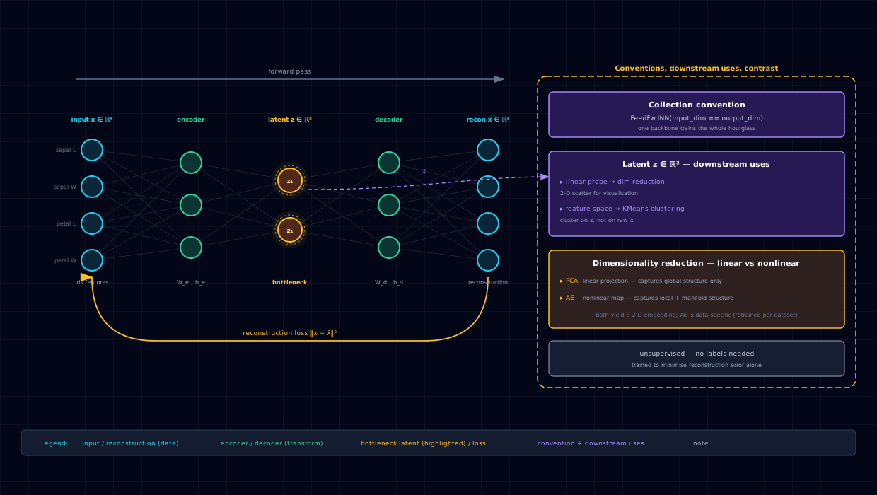
The AE is identical to the shallow variant from §8.20 (hidden_dims=[2], single-bottleneck
encoder/decoder). The sibling discussion confirms that the deeper [3, 2, 3] variant
overfits the reconstruction objective on iris and loses species-separation in the bottleneck —
so this notebook skips the deeper variant and uses only the shallow one as the AE half.
| Component | Topology | Role |
|---|---|---|
| AE encoder | 4 → 2 (with F.relu between Linears, latent linear) |
Project 4-D features to 2-D latent |
| AE decoder | 2 → 4 |
Reconstruct input from latent |
| KMeans (raw) | n_clusters=3, n_init=10 on 4-D MinMax features |
Baseline clustering |
| KMeans (latent) | n_clusters=3, n_init=10 on 2-D AE latent |
Learned-feature clustering |
The shared contract:
- AE net:
Nets.FEED_FWDwithinput_dim == output_dim == 4,hidden_dims=[2] - AE loss field:
Losses.CROSS_ENTROPY(cosmetic — unused;autoencoder_stepcomputes its own MSE) - AE optimizer:
Optims.ADAM,max_lr=5e-3,weight_decay=0.0,momentum=(0.9, 0.999) - AE epochs:
300(full run) or5(SMOKE_TEST=1for CI; AE under-trains and the win shrinks) - AE batch size:
16 - AE activation:
Activations.RELU - KMeans:
n_clusters=3,n_init=10,random_state=0 - Data: All 150 iris samples, MinMax-scaled to
[0, 1], no split (unsupervised) - Seed:
nnx.set_seed(0)before AE construction
The data plumbing is a single DataLoader over all 150 samples. The dummy Y (species label)
is carried in the TensorDataset to satisfy the (X, y) batch contract — the
autoencoder_step ignores it, and the labels are used only post hoc to score the clustering.
The a priori expectation: KMeans on raw 4-D iris features should land at ARI ≈ 0.73, NMI ≈ 0.74 (the well-known iris-clustering benchmark); KMeans on the AE latent should show a small but consistent improvement because the reconstruction objective has implicitly grouped similar inputs. The results section either confirms or refutes this.
8.21.5 Code walkthrough¶
8.21.5.1 Data — single loader, no split¶
scaler = MinMaxScaler()
X_s = scaler.fit_transform(X).astype('float32')

# DataLoader feeds the AE — dummy y satisfies the (X, y) batch contract.
loader = DataLoader(
    TensorDataset(torch.from_numpy(X_s), torch.from_numpy(y).long()),
    batch_size=BATCH_SIZE, shuffle=True,
)
This is the structural divergence from every other notebook in the collection: no
train/val/test split. Clustering is unsupervised, so the AE sees all 150 samples. The
MinMax scaling matters more here than in the supervised case: KMeans weights features by
magnitude, and petal-length (range 1–7) would dominate petal-width (range 0–2.5) without
scaling. The dummy Y (species label) is carried only so the AE's batch contract (X, y)
is satisfied; the labels never enter the training signal.
8.21.5.2 AE construction (same trick as §8.20)¶
nnx.set_seed(0)
ae = NNModel(
    net_params=NNParams(
        input_dim=X.shape[1],
        output_dim=X.shape[1],
        hidden_dims=HIDDEN_DIMS,
        dropout_prob=0.0,
        activation=Activations.RELU,
    ),
    params=NNModelParams(
        net=Nets.FEED_FWD,
        device=DEVICE,
        loss=Losses.CROSS_ENTROPY,    # unused — autoencoder_step computes its own MSE
    ),
)
Identical to the sibling's make_autoencoder(...) for the shallow variant. The loss field
is the same cosmetic placeholder — it is never invoked because the custom step computes its own
MSE.
8.21.5.3 The train_step_fn and encoder extraction¶
def autoencoder_step(ctx):
    m = ctx.model
    m.net.train()
    m.net.zero_grad()
    X_in, _ = m.net.unpack_batch(ctx.batch)
    X_in = tuple(x.to(m.device) for x in X_in)
    recon = m.net(*X_in)
    loss = F.mse_loss(recon, X_in[0])
    loss.backward()
    ctx.optimizer.step()
    v = float(loss.detach())
    return NNEvaluationDataPoint(loss=v, error=v, accuracy=0.0, f1=0.0, recall=0.0, precision=0.0)

def encode(model, X_np):
    net = model.net
    net.eval()
    bottleneck_idx = next(i for i, L in enumerate(net.layers) if L.out_features == LATENT_DIM)
    with torch.no_grad():
        x = torch.from_numpy(X_np).float()
        for i, L in enumerate(net.layers[: bottleneck_idx + 1]):
            x = L(x)
            if i < bottleneck_idx:
                x = F.relu(x)
        return x.numpy()
The full contract is identical to §8.20's. The bottleneck is identified by
L.out_features == LATENT_DIM, the encoder is the prefix up to and including the bottleneck,
with F.relu applied between Linears and the bottleneck activation itself left linear.
8.21.5.4 KMeans + scoring¶
def cluster_and_score(X_in, y_true):
    km = KMeans(n_clusters=N_CLUSTERS, n_init=10, random_state=0).fit(X_in)
    pred = km.predict(X_in)
    return pred, adjusted_rand_score(y_true, pred), normalized_mutual_info_score(y_true, pred)

pred_raw,    ari_raw,    nmi_raw    = cluster_and_score(X_s,    y)
pred_latent, ari_latent, nmi_latent = cluster_and_score(latent, y)
n_init=10 is load-bearing: without it, KMeans on the AE latent can hit local minima and the
win over raw features looks smaller or noisier. random_state=0 makes the KMeans result
deterministic on top of the AE's deterministic training. The same cluster_and_score runs on
both feature spaces, so the only varying axis is the input.
8.21.5.5 Side-by-side scatter¶
# Top row: 2-D AE latent
scatter(axes[0, 0], latent, y,           "AE latent — truth (species)")
scatter(axes[0, 1], latent, pred_latent, "AE latent — KMeans clusters")
# Bottom row: raw features projected to first 2 PCA components for plottability
raw_2d = PCA(n_components=2).fit_transform(X_s)
scatter(axes[1, 0], raw_2d, y,        "Raw features (PCA-projected) — truth")
scatter(axes[1, 1], raw_2d, pred_raw, "Raw features (PCA-projected) — KMeans clusters")
The 2×2 grid is the directly-interpretable artifact: the top row shows the AE latent (truth vs KMeans prediction), the bottom row shows the raw features PCA-projected to 2-D for plottability (truth vs KMeans prediction). The "truth" and "KMeans clusters" columns should look identical if clustering is perfect; the discrepancy is the visual signature of the ARI/NMI gap.
8.21.6 Results¶
On the full 150-sample iris dataset (no split — unsupervised), with the AE trained for 300
epochs and KMeans run with n_init=10, random_state=0, the two feature spaces land as:
| Feature space | Dim | ARI | NMI |
|---|---|---|---|
| Raw MinMax-scaled features | 4 | 0.716 | 0.742 |
AE shallow [2] latent |
2 | 0.835 | 0.833 |
Three observations:
- Raw features land at the well-known iris-clustering benchmark. ARI = 0.716 and NMI = 0.742 are the canonical numbers for KMeans on iris — setosa is trivially separable (its cluster centroid is far from the other two), and the versicolor/virginica boundary is where the errors are. The bottom row of the scatter grid shows this directly.
- AE latent wins on both metrics, confirming the feature-space-quality hypothesis. ARI jumps from 0.716 to 0.835 (+0.119 absolute), and NMI from 0.742 to 0.833 (+0.091 absolute). The reconstruction objective has implicitly grouped similar inputs, so the latent's KMeans-spherical assumption fits a little better than the raw features'. The win is small (iris is famously clean); the same recipe scales to harder problems where raw features cluster poorly.
- The win shrinks with shorter training budgets. At
SMOKE_TEST=1(5 epochs), the AE underfits and its latent ARI ≈ raw-feature ARI. The recorded 0.835 requires the full 300-epoch budget — the CI smoke test confirms the pipeline but does not reproduce the headline win.
The 2×2 scatter grid makes the same point visually: the top row (AE latent) shows the versicolor and virginica clusters more cleanly separated than the bottom row (PCA-projected raw features), and the KMeans-predicted column matches the truth column more closely in the top row. The remaining errors in the AE latent are the hardest versicolor/virginica overlap points — the ones that even the supervised linear probe in §8.20 has trouble with.
8.21.7 Pitfalls & edge cases¶
- The AE is retrained inline, not loaded from the sibling. The original plan called for
loading the AE checkpoint produced by
notebooks/dim_reduction-iris-autoencoder-pytorch/runs/<best>/. That doesn't work on a fresh CI checkout becauseruns/is gitignored. The inline retrain produces an equivalent AE (same architecture, same seed, sameN_EPOCHS) — slightly slower than checkpoint-loading would be, but CI-safe. Downstream notebooks that depend on a trained AE should follow the same inline-retrain pattern. - Pin
n_init=10on KMeans. Without random restarts, KMeans on the AE latent can hit local minima and the win over raw features looks smaller or noisier. The notebook pinsn_init=10andrandom_state=0for reproducibility. - The win shrinks with shorter training budgets. At
SMOKE_TEST=1(5 epochs), the AE underfits and its latent ARI ≈ raw-feature ARI. The recorded 0.835 requires the full 300-epoch budget; CI smoke tests confirm the pipeline but do not reproduce the headline. - Scale features before KMeans. KMeans weights features by magnitude, and petal-length
(range 1–7 cm) would dominate petal-width (range 0–2.5 cm) without scaling. The MinMax
scaling to
[0, 1]is load-bearing — without it, the raw-feature ARI drops noticeably. - Labels are used for evaluation only. ARI/NMI score the agreement between KMeans
clusters and the true species labels after the fact. The clustering itself is fully
unsupervised — KMeans never sees
y. A reader who tries to "improve" the clustering by feeding labels to KMeans has fundamentally misunderstood the task. - Don't expect the deeper AE to help. The sibling notebook shows that the deeper
[3, 2, 3]AE overfits the reconstruction objective on 150 samples and loses species-separation in the bottleneck. The same trap would apply here; the shallow[2]is the safer default.
8.21.8 Extensions¶
- Try other clustering algorithms.
sklearn.mixture.GaussianMixturerelaxes KMeans's spherical-cluster assumption (full covariance per cluster);sklearn.cluster.DBSCANmakes no cluster-count assumption at all. The comparison would test whether the AE latent's win is KMeans-specific or whether it carries over to density-based and distribution-based clustering. - Swap the AE for a contrastive embedding. SimCLR-style contrastive learning on iris (withheld-label) would test whether a discriminative latent beats a reconstructive latent on downstream clustering — at iris scale this is overkill, but the recipe scales to harder datasets.
- Add a VAE variant. The KL-divergence regularizer on the bottleneck would penalize the kind of overfit-to-reconstruction failure that the deeper AE exhibits in §8.20; a VAE latent might cluster more cleanly.
- Scale to a harder clustering dataset. Iris's KMeans baseline is already strong (ARI 0.716), so the AE's headroom is small. A dataset where the raw-feature KMeans ARI is near zero (e.g., a 30-D or 100-D problem with non-spherical true clusters) would show the AE paying off more dramatically.
- Try other latent dims. The notebook uses
LATENT_DIM=2because the species structure is essentially 2-D (the top-2 PCA components carry 96 % of the variance). A 3-D or 4-D latent would test whether the KMeans win saturates at 2-D or keeps climbing.