8.6 Knowledge distillation — MNIST FFN (born-again)¶
A comprehensive walk-through of notebooks/knowledge_distillation-mnist-ffnn-pytorch/ — the
canonical in-repo demo of nnx.born_again_train and the born-again (same-architecture
self-distillation) pattern. This page is the deep-dive companion to the task notebook: it states
the problem, builds the distillation math, dissects the born-again iteration, reads the code top to
bottom, reports the measured per-generation trajectory, and catalogues the pitfalls and extensions.
The notebook is Tier-A — CPU re-runs in roughly 25 seconds and it is re-executed end-to-end in CI on every pull request. It belongs to the "efficient/compressed MLP" family: where §8.5 changes the architecture and §8.7/§8.8 change the sparsity/bitwidth, born-again distillation keeps the parameter count fixed and instead changes what the model is trained against — soft labels from a frozen copy of itself.
The committed metrics are preserved NNx 0.2.0-era evidence. Issue #61 executed 0.2.2 only into temporary artifacts and retained 0.2.0 for the recommended Atlas runtime; this page does not attribute the checked-in results to the rejected pin trial.
8.6.1 Problem & motivation¶
Knowledge distillation (Hinton et al., 2015) trains a student model to match a teacher's soft predictions, not just the hard labels. The original use case was compression: a small student learns from a big teacher and approaches the teacher's accuracy at a fraction of the parameter count. Born-again training (Furlanello et al., 2018) is the surprising special case where student and teacher have the same architecture: each "generation" copies the previous generation's frozen weights as its teacher. Empirically, BA-\(k\) often beats single-generation training despite the identical parameter count — the gain comes entirely from the soft-label regularizer.
This notebook exists for two reasons:
- First in-repo exercise of
nnx.born_again_train. Thennxrelease ships a single call that wires the iterated-distillation loop; this notebook is the canonical demo of the contract and its per-generation convergence consequences on a real trained model. - The born-again result is counterintuitive and worth seeing directly. A student with no extra data and (modulo soft labels) no extra information beating its teacher is a claim most readers will not believe until they see the trajectory. The notebook shows the per-generation validation loss falling monotonically across three generations.
The falsifiable hypothesis tested by the notebook is that a 3-generation born-again chain reaches higher validation accuracy than a single-generation reference trained from the same fresh init under the same per-generation epoch budget.
8.6.2 Concepts¶
| Concept | Where it shows up |
|---|---|
| Knowledge distillation | Student trained against teacher's soft predictions, not just hard labels |
| Born-again (self-distillation) | Same-architecture teacher; each generation teaches the next |
| Soft labels / dark knowledge | The teacher's softmax distribution carries inter-class structure hard labels lack |
| Temperature softmax | Sharpens/softens the teacher distribution (the regularization knob) |
| Frozen teacher | Teacher weights are deepcopy'd, .eval(), requires_grad=False |
| Per-generation trajectory | val loss should fall monotonically across generations |
nnx.FeedFwdNN (Nets.FEED_FWD) |
The shared student/teacher architecture; [128, 64] |
| Reproducibility | nnx.set_seed(0) pins Python random, NumPy, PyTorch CPU + CUDA + cuDNN |
The nnx surface consumed is: NNModel, NNParams, NNModelParams, NNTrainParams,
NNOptimParams, NNDataset, Activations, Devices, Losses, Nets, Optims, set_seed, and
the distillation primitive nnx.born_again_train (which internally uses
nnx.kd_train_step_factory(teacher=...)).
8.6.3 Mathematical formulation¶
A standard classifier is trained against the one-hot label \(y\) with cross-entropy on the softmax distribution. In distillation, the student is additionally trained against the teacher's softmax distribution \(p^T\). The teacher's softmax is computed at a temperature \(T > 1\), which softens it and exposes the "dark knowledge" — the small probabilities the teacher assigns to non-target classes that encode which mistakes are near-misses:
The student is trained to match this softened distribution (also at temperature \(T\)) via a second cross-entropy term, typically combined with the hard-label cross-entropy at a small weight:
The \(T^2\) factor preserves the gradient magnitude as \(T\) scales the logits (a Hinton et al.
detail; nnx.kd_train_step_factory handles the scaling internally).
Born-again is the recursion: let \(M_0\) be a model trained plain on hard labels (gen 0). For \(k = 1, 2, \dots\), train \(M_k\) by distilling from a frozen copy of \(M_{k-1}\):
Two details matter. First, the live model is reused in place across generations — its weights are
not reset between generations, so gen \(k\) continues training the same network that gen \(k-1\)
produced. Second, the teacher is a separate deepcopy of the gen \(k-1\) snapshot, frozen via
.eval() and requires_grad=False. So the only thing varying across generations is what the live
model is trained against: hard labels (gen 0) vs soft-from-frozen-prior (gen \(k > 0\)).
The original paper showed BA-\(k\) students often beat their teachers on ResNet-110/CIFAR-100, with gains tapering past BA-4. The accepted explanation is that the teacher's softened distribution acts as a label-smoothing regularizer — it tells the student which confusions are near-misses vs catastrophic, and this targeted smoothing improves generalization at no extra parameter cost.
8.6.4 Architecture¶
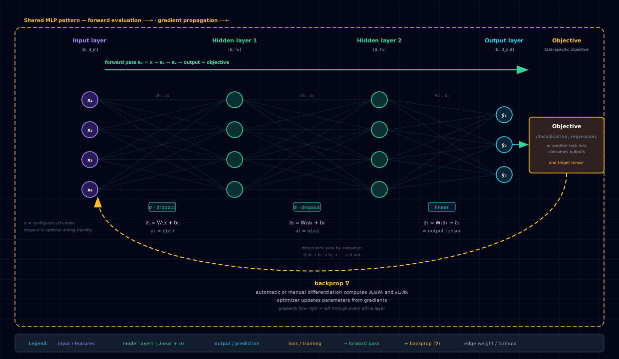
The architecture is Nets.FEED_FWD (nnx.FeedFwdNN): a 784-unit input layer (flattened MNIST),
two hidden layers [128, 64] with ReLU, and a 10-unit output layer consumed by softmax +
cross-entropy. Crucially, the same architecture is used for student and teacher — that is the
born-again constraint.
| Object | hidden_dims |
Role |
|---|---|---|
| Single-gen reference | [128, 64] |
Trained plain on hard labels; the control |
| Born-again gen 0 | [128, 64] |
Trained plain on hard labels (same as single-gen) |
| Born-again gen 1 | [128, 64] |
Distills from a frozen copy of gen 0 |
| Born-again gen 2 | [128, 64] |
Distills from a frozen copy of gen 1 |
The shared contract — identical for the single-gen reference and every born-again generation:
- Net:
Nets.FEED_FWD, activation:Activations.RELU - Loss:
Losses.CROSS_ENTROPY - Optimizer: Adam,
max_lr=1e-3,weight_decay=0.0,momentum=(0.9, 0.999) - Device:
Devices.CPU - Budget:
N_EPOCHS=2per generation,N_GENERATIONS=3(orSMOKE_TEST_EPOCHS=1/SMOKE_TEST_GENS=2underSMOKE_TEST=1) - Seed:
0, re-pinned before both the single-gen reference and the born-again chain so both start from the same fresh init - Batching:
batch_sizes=(128, None, None)— 128-sample train minibatches; val as one batch
The a priori expectation: gen 0 should match the single-gen reference exactly (same init, same data, same budget), and gens 1–2 should improve monotonically as the soft-label regularizer compounds. Whether the absolute accuracy is high or low is a function of the 2-epoch budget; the direction of the per-generation trajectory is the pedagogically interesting signal.
8.6.5 Code walkthrough¶
8.6.5.1 Model and training-parameter factories¶
def make_model():
    return NNModel(
        net_params=NNParams(
            input_dim=ds.input_dim, output_dim=ds.output_dim,
            hidden_dims=HIDDEN_DIMS, dropout_prob=0.0,
            activation=Activations.RELU,
        ),
        params=NNModelParams(net=Nets.FEED_FWD, device=DEVICE, loss=Losses.CROSS_ENTROPY),
    )

def train_params():
    return NNTrainParams(
        n_epochs=N_EPOCHS,
        train_loader=ds.train_loader, val_loader=ds.val_loader,
        optim=NNOptimParams(name=Optims.ADAM, max_lr=LR,
                            momentum=(0.9, 0.999), weight_decay=0.0),
    )
Both factories are pure — each call returns a fresh object — so the single-gen reference and the
born-again chain can be built from identical starting conditions. dropout_prob=0.0 because the
budget is tiny and dropout would starve an already-undertrained model.
8.6.5.2 Single-generation reference¶
nnx.set_seed(0)
single_gen = make_model()
single_run = single_gen.train(params=train_params())
print(f"single-gen: final val_loss={single_run.idps[-1].val_edp.loss:.4f}")
This is the control. With set_seed(0) immediately before, and make_model() + train_params()
deterministic, the reference's final recorded validation loss is 2.1403 (validation accuracy
40.73% — low, because the budget is 2 epochs).
8.6.5.3 Born-again chain — one call¶
nnx.set_seed(0)
ba_model = make_model()
ba_runs = nnx.born_again_train(
    ba_model,
    generations=N_GENERATIONS,
    train_params=train_params(),
)
born_again_train returns a list[NNRun] of length N_GENERATIONS. The single ba_model object
is reused in place across all generations: its weights carry over from gen to gen, and only the
teacher is a separate frozen deepcopy of the prior-gen snapshot. So after the call returns,
ba_model holds the last generation's parameters and ba_runs[i].idps[-1].val_edp.loss is gen
\(i\)'s final validation loss.
8.6.5.4 Per-generation trajectory¶
for i, run in enumerate(ba_runs):
    trained_against = "hard labels" if i == 0 else f"frozen gen {i-1} (soft)"
    t2.add_row([i, trained_against, f"{run.idps[-1].val_edp.loss:.4f}"])
The trajectory table is the directly-interpretable artifact: it pairs each generation's final validation loss with what that generation was trained against, making the soft-label handoff explicit.
8.6.5.5 Final comparison¶
single_acc = single_gen.evaluate(ds.val_loader).accuracy
ba_acc = ba_model.evaluate(ds.val_loader).accuracy
# table: single-gen vs born-again gen (N-1), val loss + val acc
model.evaluate(ds.val_loader) runs one forward pass over the held-out validation split and returns
an evaluation data point carrying accuracy. The verdict compares the single-gen reference against
the born-again chain's final generation (gen 2), which is the one whose weights live in
ba_model after the call.
8.6.6 Results & analysis¶
On the recorded (seeded) run, the single-gen reference and the 3-generation born-again chain land as:
| Recipe | Final val loss | Val accuracy |
|---|---|---|
| single-gen (cross-entropy only) | 2.1403 | 40.73% |
| born-again gen 2 (last) | 1.6501 | 62.07% |
Per-generation trajectory:
| Generation | Trained against | Final val loss |
|---|---|---|
| 0 | hard labels | 2.1403 |
| 1 | frozen gen 0 (soft) | 1.9074 |
| 2 | frozen gen 1 (soft) | 1.6501 |
Three observations:
- Gen 0 matches the single-gen reference exactly. Both start from
set_seed(0)+ the samemake_model()init and train on hard labels for the same 2 epochs, so they produce identical weights and identical validation loss (2.1403). This confirms the controlled-comparison framing — the only thing that differs in gens 1–2 is the soft-label handoff. - Validation loss falls monotonically across generations (2.14 → 1.91 → 1.65), and the final born-again generation reaches 62.07% validation accuracy versus the single-gen reference's 40.73% — a +21-point gain at the same parameter count. This is the born-again headline made visible.
- The gain's magnitude is inflated by the tiny budget. Each generation gets only 2 epochs, so the single-gen baseline is badly undertrained and each extra generation is partly just more total optimization (the live weights carry over and keep training) rather than a pure soft-label effect. The §6.3 discussion cell is explicit about this confound. At longer budgets the per-generation improvement compounds for a few generations before plateauing — diminishing returns past BA-4 or so in the original paper.
The right reading is therefore: the soft-label regularizer has a real, free generalization gain at fixed parameter count (the direction of the trajectory is the signal), and the absolute gap is budget-confounded (the magnitude is not pure distillation). Both are honest.
8.6.7 Pitfalls & edge cases¶
- Short budget inflates the born-again gap. The +21-point recorded jump is partly "more total optimization" because the live model carries weights over across generations. To isolate the pure soft-label effect, train each generation to a fixed accuracy target rather than a fixed epoch count, or compare against a single-gen baseline trained for the total epoch budget of the whole chain (here, 6 epochs). The notebook's §6.3 calls this out; do not present the headline number as a pure distillation gain.
- Diminishing returns past ~BA-4. The original paper shows gains taper off on
ResNet-110/CIFAR-100. This notebook runs only 3 generations to stay Tier-A, so the plateau is
not visible. Extending
N_GENERATIONSpast 5 is unlikely to help and costs Tier-A time. - Same-architecture only. Born-again intentionally fixes the student to the same
architecture as the teacher. The classical compression case (small student, big teacher) uses
the same
nnx.kd_train_step_factory(teacher=...)plumbing but with differentNNParamsfor student and teacher — that is a different notebook's scope. - The live model is reused in place.
ba_modelafter the call holds gen \(N-1\)'s weights, not gen 0's. If you want to keep an earlier generation's model,deepcopyit before the next generation starts;born_again_traindoes not retain intermediate live models (only theNNRunhistory objects). - Re-pin the seed before both runs.
set_seed(0)is called before the single-gen reference and before the born-again chain so both start from identical inits. Without the re-pin, the RNG state advances between the two top-level calls and the gen-0-vs-single-gen match (the controlled-comparison sanity check) breaks. - The teacher must be frozen.
born_again_trainhandles the.eval()+requires_grad=Falseinternally, but if you usennx.kd_train_step_factory(teacher=...)directly, forgetting to freeze the teacher silently trains it in lockstep with the student and the distillation signal collapses to self-training. - Per-generation epoch count vs total.
N_EPOCHS=2is per generation, so the born-again chain sees \(3 \times 2 = 6\) epochs of live-weight training while the single-gen reference sees - This is the same confound as pitfall #1; state it explicitly when reporting results.
8.6.8 Extensions & references¶
- Control for the budget confound. Compare born-again gen 2 against a single-gen baseline trained for the total epoch budget of the chain (6 epochs at 2 per generation). The remaining gap is the pure soft-label effect; the rest is extra optimization. This is the cleanest way to report a distillation gain.
- Extend to the compression case. Swap the student's
NNParamsfor a smaller architecture (e.g.[32, 16]) while keeping the teacher at[128, 64], using the samennx.kd_train_step_factory(teacher=...)plumbing. This is the classical Hinton-style compression and the original motivation for distillation. - Vary the temperature and distillation weight. \(\lambda\) and \(T\) are the two knobs on the distillation loss; sweep them and plot validation accuracy as a 2-D surface. Low \(T\) approximates hard labels; high \(T\) over-softens and the signal vanishes.
- Run more generations to find the plateau. The original paper shows gains tapering past BA-4;
set
N_GENERATIONS=6(and drop back to Tier-B/longer runtime) to see the plateau directly on MNIST. - References. Furlanello et al., 2018, Born-Again Neural Networks (arXiv:1805.04770) — the
same-architecture self-distillation result. Hinton et al., 2015, Distilling the Knowledge in a
Neural Network (arXiv:1503.02531) — the original distillation framework with the temperature
formulation. See also the task
README.mdfor the in-repo contract summary anddocs/env-setup.md§4.1.6 for the Tier-A execution path.