8.13 Node classification — Reddit GNN¶

A comprehensive walk-through of notebooks/node_classification-reddit-gnn-pyg/ — the lab's largest graph task and the canonical vehicle for the message-passing model family (GraphConv, GraphSAGE, GraphAttention) alongside a feature-only feed-forward baseline. This page is the deep-dive companion to the task's nine notebooks: it states the problem, builds the message-passing math, dissects the three-phase experimental flow, reads the code top to bottom, reports the measured results, and catalogues the pitfalls and extensions that govern graph-structural learning at scale.

The task is Tier-B/C — Phase 1 and Phase 2 smoke-run to /tmp under make smoke-tier-b, but Phase 3's full training runs are multi-day CPU jobs whose August-2023 outputs are preserved in place (Tier-C, do not re-execute). Issue #61 completed both smoke tiers on clean Darwin arm64 with torch_sparse==0.6.18; platform assumptions do not waive either release-review tier.

The committed Reddit results remain preserved historical outputs. Issue #61's 0.2.2 Tier B/C execution wrote only fresh temporary artifacts; the final checked-in source retains the Atlas-compatible NNx 0.2.0 call surface.

8.13.1 Problem & motivation¶

Reddit2 is a post-to-subreddit graph: each node is a post, each edge connects posts that a shared user commented on, and the label is the subreddit community the post belongs to. The dataset shipped by PyTorch Geometric contains 232,965 nodes, 23,213,838 edges, a 602-dimensional bag-of-words / pooled-embeddings feature vector per node, and 41 classes. The graph is undirected, has no self-loops, contains a handful of isolated nodes, and has an average degree of about 99.65 — dense enough for community structure to be informative, sparse enough (density around \(3.6 \times 10^{-4}\) on a 5,000-node slice) that full-neighborhood propagation is tractable only under sampling.

This task exists for four research questions, one per Phase-3 notebook:

How does a feature-only feed-forward network perform on node classification with a large graph?
Can a Graph Convolutional Network outperform the FFN, and at what computational cost?
How does GraphSAGE compare to GCN and the FFN?
What does the attention mechanism (GAT) add?

The falsifiable hypothesis running through the three phases: graph-structural neighborhood signal should beat the feature-only baseline by a wide margin on a graph this dense, and the question is which message-passing flavor wins and how deep it should be. Phase 1 characterizes the graph; Phase 2 sweeps architectures and hyperparameters over short budgets; Phase 3 trains the survivors to convergence.

8.13.2 Concepts¶

Concept	Where it shows up
Node classification	Predict the subreddit label of each post node (41 classes)
Message passing	The unifying abstraction: each layer aggregates from the 1-hop neighborhood
GraphConv (GCN)	`Nets.GRAPH_CONV` — symmetrically-scaled spectral propagation
GraphSAGE	`Nets.GRAPH_SAGE` — sampled-neighborhood aggregator (mean); depth-tolerant
Graph Attention (GAT)	`Nets.GRAPH_ATT` with `n_heads` — learned, asymmetric neighbor weights
NeighborLoader sampling	`[20, 15, 10]` fanout per hop — makes full-Reddit training fit on one CPU
Transductive splits	Reddit2 ships fixed `train_mask` / `val_mask` / `test_mask` (66/10/24%)
Louvain community detection	Phase 1 sanity check: does the graph recover the 41 subreddits?
t-SNE projection	Phase 1 feature visualization; Phase 2/3 checkpoint-logit visualization
Seed-node evaluation	`model.evaluate(loader)` scores only seed nodes — sampled neighbors leak cross-split labels
Deterministic graph sampling	`SEED = 0`; public `set_seed(SEED)` immediately before each `NNGraphDataset(...)` construction

The nnx flat re-exports consumed are: NNGraphDataset, NNModel, NNParams, NNModelParams, NNTrainParams, NNOptimParams, NNRun, Devices, Losses, Nets, Optims, VisUtils, Utils, set_seed. The graph-aware enums (Nets.GRAPH_CONV, Nets.GRAPH_SAGE, Nets.GRAPH_ATT) are paired with NNParams(hidden_dims=..., dropout_prob=..., n_heads=...); only GRAPH_ATT consumes n_heads. GraphConvNN wraps pyg.nn.GCNConv; the collection name does not refer to PyG's separate pyg.nn.GraphConv operator.

8.13.3 Math¶

The unifying abstraction for all three message-passing variants is the per-layer update of node \(v\)'s representation by combining its own features with an aggregation over its neighborhood \(\mathcal{N}(v)\):

\[ h_v^{(k)} = \phi\!\left(W^{(k)} h_v^{(k-1)} \;\oplus\; \bigoplus_{u \in \mathcal{N}(v)} \psi^{(k)}(h_u^{(k-1)})\right), \]

with \(h_v^{(0)} = x_v\) (the 602-dim input feature) and the readout on layer \(K\) producing 41 logits consumed by softmax + cross-entropy (same objective as the Iris task in §8.1).

GraphConv (Kipf & Welling) uses a symmetrically normalized sum over the closed neighborhood, where the normalization is the inverse square root of the endpoint degrees:

\[ h_v^{(k)} = \sigma\!\left(\sum_{u \in \mathcal{N}(v) \cup \{v\}} \frac{1}{\sqrt{d_u\, d_v}}\, W^{(k)} h_u^{(k-1)}\right). \]

GraphSAGE concatenates the self representation with an independently-weighted neighborhood aggregation (mean aggregator here) and applies the activation after the linear map:

\[ h_v^{(k)} = \sigma\!\left(W^{(k)} \cdot \mathrm{CONCAT}\!\left(h_v^{(k-1)},\; \mathrm{MEAN}_{u \in \mathcal{N}(v)}(h_u^{(k-1)})\right)\right), \qquad h_v^{(k)} \leftarrow \frac{h_v^{(k)}}{\|h_v^{(k)}\|_2}. \]

The per-node L2 renormalization is load-bearing on a graph whose degrees span four orders of magnitude — without it, high-degree hubs dominate the next layer.

Graph Attention (GAT) replaces the fixed \(1/\sqrt{d_u d_v}\) weight with a learned, content-addressable coefficient \(\alpha_{vu}\) computed from a shared attention vector \(\mathbf{a}\) over the linearly-projected endpoint features:

\[ \alpha_{vu} = \frac{\exp\!\left(\mathrm{LeakyReLU}\!\left(\mathbf{a}^\top [\mathbf{W}h_v \| \mathbf{W}h_u]\right)\right)}{\sum_{w \in \mathcal{N}(v)} \exp\!\left(\mathrm{LeakyReLU}\!\left(\mathbf{a}^\top [\mathbf{W}h_v \| \mathbf{W}h_w]\right)\right)}, \qquad h_v^{(k)} = \sigma\!\left(\sum_{u \in \mathcal{N}(v)} \alpha_{vu}\, \mathbf{W} h_u^{(k-1)}\right). \]

The Phase-3 GAT uses n_heads=4 attention heads whose outputs are concatenated; multi-head attention stabilizes the softmax-over-neighborhood by averaging over independently-initialized \(\mathbf{a}\) vectors.

8.13.4 Architecture¶

GNN message-passing

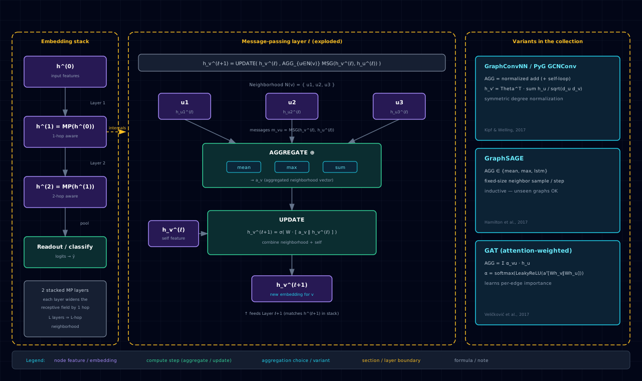
Because this is a multi-phase investigation, the "architecture" story is the phase flow itself: Phase 1 understands the graph, Phase 2 narrows the model space, Phase 3 trains the survivors to convergence. The candidate architectures compared across phases:

Family	`nnx` net	Neighborhood treatment	Depth-tolerance
Feed-forward baseline	`Nets.FEED_FWD`	None (features only)	n/a — the floor to beat
GraphConv (GCN)	`Nets.GRAPH_CONV`	Full symmetric normalization	Degrades past 2 layers
GraphSAGE	`Nets.GRAPH_SAGE`	Sampled mean aggregation	Tolerates 4-6 layers
Graph Attention (GAT)	`Nets.GRAPH_ATT`	Learned attention weights	Memory-bound at width ≥ 256

Phase 1 — dataset exploration (phase1-dataset-exploration-notebook.ipynb). No training. Loads Reddit2 via torch_geometric.datasets.Reddit2(root="./data"), applies NormalizeFeatures + ToSparseTensor transforms, inspects the feature and label tensors as pandas DataFrames, takes a 5,000-node prefix slice (the first-N-rows subgraph), converts it to NetworkX, renders it colored by ground-truth labels and by Louvain-detected communities, and plots the degree distribution plus a log-log rank plot. The t-SNE projection of the node features is the qualitative baseline: if features alone already separate the 41 classes, the FFN baseline should be competitive; if they don't, graph structure should win. The degree distribution confirms power-law behavior, justifying the L2-normalization in SAGE and the sampling in NeighborLoader.

Phase 2 — model selection (four notebooks, short budgets). All four use NNGraphDataset(ds_class=pyg.datasets.Reddit2, n_neighbors=[20, 15, 10], n_workers=4, transform=Compose([NormalizeFeatures()])) and Devices.CPU. Each path defines SEED = 0 and calls public set_seed(SEED) immediately before construction.

Notebook 1 — a 16-combination grid: 4 architectures × 2 learning rates \((10^{-2}, 10^{-4})\) × 2 dropouts \((0.25, 0.5)\), single hidden layer [128], 100 epochs, Adam with weight_decay=5e-4, momentum=(0.9, 0.999). GAT wins at lr=1e-4, dropout=0.25 (validation error 0.3255); the FFN baseline finishes last (validation error 0.67+).
Notebook 2 — 500-epoch convergence study of all four at the matched config ([128], lr=1e-2, dropout=0.25). GAT still leads (validation error 0.2521); GraphSAGE and GraphConv track each other; the FFN plateaus early, confirming graph structure is essential.
Notebook 3 — deep/wide architecture test: hidden [1024, 512, 256] (3 layers), 250 epochs, lr=1e-4, dropout=0.5. GAT is excluded — it hit GPU-memory ceilings on the original training hardware at width ≥ 256. GraphSAGE wins (validation error 0.4452); GraphConv scales poorly with full-neighborhood processing at this depth.
Notebook 4 — a single-architecture GAT deep-dive: n_heads=5, hidden [512, 256, 128, 64], 1000 epochs, dropout=0.5. This is a convergence study, not a sweep; the markdown records a target validation error around 0.2232, but the training cell outputs are not preserved in the committed notebook, so the number is prose-only.

Phase 3 — final training and evaluation (four notebooks, Tier-C). Each takes the Phase-2 pick for one architecture to a long-horizon run. The shared contract: n_neighbors=[20, 15, 10], weight_decay=5e-4, momentum=(0.9, 0.999), Adam, cross-entropy, Devices.CPU, and set_seed(SEED) with SEED = 0.

Notebook	Model	`hidden_dims`	`dropout_prob`	`max_lr`	Epochs	Role
1	GAT (`n_heads=4`)	`[128]`	0.25	\(10^{-2}\)	1200	Phase-2 GAT winner, converged
2	GraphSAGE depth-1	`[1024, 512, 256, 128]`	0.5	\(10^{-4}\)	2000	First SAGE depth probe
3	GraphSAGE depth-2	`[1024, 512, 256, 128, 64]`	0.5	\(10^{-4}\)	2000	Added layer
4	GraphSAGE depth-3	`[768, 1024, 512, 256, 128, 64]`	0.5	\(10^{-4}\)	2000	Non-monotone first-layer width

The GAT run uses a 100× larger learning rate than the GraphSAGE runs because GAT's attention normalization keeps gradient magnitudes well-scaled; the SAGE runs at lr=1e-2 diverged in Phase-2 pilot runs, hence the drop to 1e-4. The depth-3 notebook uses a narrower first layer (768 < 1024) to test whether a non-monotone width funnel helps once the receptive field is large.

8.13.5 Code walkthrough¶

8.13.5.1 Phase 1 — loading and exploring the graph¶

dataset = pyg.datasets.Reddit2(
    root="./data",
    transform=pyg.transforms.Compose([
        pyg.transforms.NormalizeFeatures(),
        pyg.transforms.ToSparseTensor(remove_edge_index=False),
    ]),
)

NormalizeFeatures row-normalizes the 602-dim feature matrix so posts with very different comment volumes are comparable; ToSparseTensor packs the edge index for fast propagation. Phase 1 then converts a prefix slice to NetworkX and compares ground-truth labels against Louvain communities — the qualitative read on whether the graph alone (ignoring features) recovers the 41 subreddits.

8.13.5.2 Phase 2/3 — graph dataset plumbing¶

SEED = 0
set_seed(SEED)
ds = NNGraphDataset(
    ds_class=pyg.datasets.Reddit2,
    n_neighbors=N_NEIGHBORS,            # [20, 15, 10]
    n_workers=4,
    transform=pyg.transforms.Compose([pyg.transforms.NormalizeFeatures()]),
)
train_loader = ds.train_loader
val_loader   = ds.val_loader
test_loader  = ds.test_loader

NNGraphDataset is the graph analogue of NNTabularDataset: it wraps a PyG dataset class and constructs three NeighborLoader iterators internally — one per split mask. The n_neighbors=[20, 15, 10] argument is the per-hop fanout: each seed node samples up to 20 first-hop neighbors, 15 second-hop, and 10 third-hop, which bounds the receptive field so that full-Reddit training fits in memory on one CPU. ds.input_dim is 602 and ds.output_dim is 41, sourced from the dataset object.

This ordering is deliberate. Released thekaveh-nnx==0.2.0 does not accept NNGraphDataset(seed=...); its NeighborLoader(shuffle=True, ...) consumes the global Torch RNG. The public set_seed(SEED) call is therefore repeated immediately at the construction boundary. The NNx-surface suite rejects missing, dead-code, non-adjacent, or unsupported constructor seeding and executes a tiny graph twice to prove that the first sampled batch repeats.

8.13.5.3 Phase 2 — the candidate grid¶

net_specs = [
    (Nets.GRAPH_ATT,  n_heads := 4),
    (Nets.GRAPH_SAGE, None),
    (Nets.GRAPH_CONV, None),
    (Nets.FEED_FWD,   None),
]
hidden_dimss = [[128]]
lrs          = [1e-2, 1e-4]
dropout_probs = [0.25, 0.5]

for net_enum, heads in net_specs:
    for hidden_dims in hidden_dimss:
        for dropout_prob in dropout_probs:
            for lr in lrs:
                model = NNModel(
                    params=NNModelParams(net=net_enum, device=Devices.CPU,
                                         loss=Losses.CROSS_ENTROPY),
                    net_params=NNParams(n_heads=heads, hidden_dims=hidden_dims,
                                        dropout_prob=dropout_prob,
                                        input_dim=ds.input_dim, output_dim=ds.output_dim),
                )
                run = model.train(params=NNTrainParams(
                    n_epochs=n_epochs,
                    optim=NNOptimParams(name=Optims.ADAM, max_lr=lr,
                                        weight_decay=5e-4, momentum=(0.9, 0.999)),
                ).with_train_loader(value=train_loader).with_val_loader(value=val_loader))
                trains[str(run)] = (model, run.idps)

The four-way product is the 16-combination sweep of Notebook 1. NNParams is where topology lives (hidden_dims, dropout_prob, n_heads); NNModelParams carries the loss + device contract; NNOptimParams carries the optimizer. The ranking keys trains by str(run) (the model's printed signature, e.g. GraphAttNN={dims=[602, 128, 41], dropout=0.25, heads=4}) and sorts by the minimum validation error across all iteration data points:

top_model_names = sorted(
    trains.items(),
    key=lambda kvp: min(idp.val_edp.error for idp in kvp[1][1] if idp.val_edp is not None,
                        default=inf),
)[:10]

Each idp exposes .iter_idx, .train_edp (.loss, .error), .val_edp (.loss, .error), and (in Notebook 4) .lr for learning-rate plots.

8.13.5.4 Phase 3 — long-horizon training and seed-node evaluation¶

set_seed(0)
model = NNModel(
    params=NNModelParams(net=Nets.GRAPH_SAGE, device=Devices.CPU,
                         loss=Losses.CROSS_ENTROPY),
    net_params=NNParams(dropout_prob=0.5, hidden_dims=[1024, 512, 256, 128],
                        input_dim=ds.input_dim, output_dim=ds.output_dim),
)
run = model.train(params=NNTrainParams(
    n_epochs=2000,
    optim=NNOptimParams(name=Optims.ADAM, max_lr=1e-4,
                        weight_decay=5e-4, momentum=(0.9, 0.999)),
).with_train_loader(value=train_loader).with_val_loader(value=val_loader))

test_edp = model.evaluate(test_loader)
# test_edp.accuracy, test_edp.f1, test_edp.recall, test_edp.precision

Two Phase-3 details are load-bearing. First, evaluation is seed-node-only: the NeighborLoader places seed nodes first in each batch, and model.evaluate scores only those via GraphNNBase.seed_count(batch). Scoring the sampled neighbors too would leak labels from other splits and inflate metrics — the comments in the Phase-3 cells call this out explicitly as the fix for an earlier unpack_batch path that did exactly that. Second, the metrics (accuracy, f1, recall, precision) come back identical because evaluate reports micro-averages over the 41-class seed-node test set, where micro-f1 reduces to accuracy.

8.13.5.5 Convergence and checkpoint visualization¶

VisUtils.multi_line_plot(
    x=list(range(max_iters + 1)),
    yss_legend=[model_names, ["Training", "Validation"]],
    yss=[[ [idp.train_edp.error for idp in trains[name][1]],
           [idp.val_edp.error  for idp in trains[name][1]] ] for name in model_names],
    x_axis_label="Iteration", y_axis_label="Error",
    title="Training & validation error — architecture comparison",
)

Phase-2 Notebooks 1-3 overlay candidates on one figure for direct comparison. Phase-3 Notebook 4 additionally uses VisUtils.two_dim_tsne_checkpoint_logits(checkpoint=..., ds=ds, n_samples=10000) to project the checkpoint logits at the FIRST / Q1 / Q2 / Q3 / LAST iterations, showing how class separability evolves over training.

8.13.6 Results¶

8.13.6.1 Phase 2 — model selection winners (best validation error)¶

Notebook	Sweep	Winner	Best val error
1	16-combo, `[128]`, 100 epochs	GAT (`lr=1e-4`, `dropout=0.25`)	0.3255
2	4-arch convergence, 500 epochs	GAT (`lr=1e-2`, `dropout=0.25`)	0.2521
3	Deep `[1024,512,256]`, 250 epochs (GAT excluded)	GraphSAGE (`lr=1e-4`, `dropout=0.5`)	0.4452
4	GAT 1000-epoch deep-dive	GAT (`n_heads=5`)	~0.2232 (prose only — outputs not preserved)

The Phase-2 verdict: GAT dominates on narrow architectures given enough epochs, but its memory cost rules it out at width ≥ 256; GraphSAGE is the only architecture that benefits from depth, which sets up the Phase-3 depth sweep.

8.13.6.2 Phase 3 — final training and evaluation (recorded outputs)¶

Notebook	Model	Final train error	Best val error	Test accuracy
1	GAT `[128]`, heads=4, 1200 epochs	0.2457	0.2291	0.7666
2	GraphSAGE depth-1 `[1024,512,256,128]`, 2000 epochs	0.1078	0.1019	0.9055
3	GraphSAGE depth-2 `[1024,512,256,128,64]`, 2000 epochs	0.1048	0.1024	0.9094
4	GraphSAGE depth-3 `[768,1024,512,256,128,64]`, 2000 epochs	0.0943	0.0904	0.9164

Four observations:

Graph structure is decisive. The GraphSAGE runs reach ~0.91 test accuracy versus the feature-only FFN baseline's Phase-2 plateau around 0.62-0.67 error — a gap of roughly twenty-plus percentage points that confirms the central hypothesis.
GraphSAGE dominates GAT on this graph. The GAT final run (0.7666) trails every GraphSAGE depth by ~14 points. The comparison is not perfectly clean — GAT uses a 100× larger learning rate and 800 fewer epochs — but the Phase-2 evidence that GAT scales poorly at width also holds here.
Depth helps, with diminishing returns. Each added GraphSAGE layer improves both validation error and test accuracy, but the test-accuracy gain shrinks from +0.014 (depth-1 → depth-2) to +0.007 (depth-2 → depth-3). The depth-3 variant's non-monotone first-layer width (768 < 1024) edges out depth-2 on this run; whether that generalizes is open.
GAT is the runtime bottleneck. Wall times on the original M1 Max hardware range from ~16.7h (GAT, 1200 epochs) to ~56.4h (GraphSAGE depth-3, 2000 epochs), which is why Phase 3 is Tier-C with preserved outputs.

8.13.7 Pitfalls¶

GAT hits a memory ceiling at width ≥ 256. Phase-2 Notebook 3 excludes GAT entirely for this reason; Phase-3 Notebook 1 holds GAT at [128] to stay feasible. Any GAT revival needs sparsified attention (see Extensions) or a GPU with substantially more VRAM than the original M1 Max.
Score seed nodes only. The NeighborLoader puts seed nodes first in each batch and fills the rest with sampled neighbors drawn from any split. Scoring the whole batch leaks cross-split labels and inflates metrics — the Phase-3 cells enforce seed-node-only scoring via GraphNNBase.seed_count(batch), and the comments document the earlier unpack_batch path that got this wrong.
Do not re-execute Phase-3 in place. The four Tier-C notebooks carry preserved August-2023 outputs (training curves, tqdm bars, test-accuracy prints) that are part of the experimental record. make smoke-tier-c writes to /tmp/; papermill phase3-*.ipynb phase3-*.ipynb in place destroys them. The immutable tier-c-deterministic-seeding-atlas-baseline-2026-08-22 git tag enforces code-cell source equality (markdown and outputs are not compared, so markdown edits are safe). The historical pre-cleanup-baseline remains an unchanged rollback anchor.
Run both graph tiers during release review. Issue #62 requires mandatory zero-skip graph tests plus Tier B and Tier C execution on the supported Torch 2.11 CPU stack. Sampling must prove preferred pyg-lib selection and forced torch-sparse fallback; install with make install-torch-stack and prove with make verify-torch-stack.
Seed through the released public API. NNx 0.2 has no NNGraphDataset(seed=...) keyword. Define one literal SEED = 0 and call set_seed(SEED) immediately before construction; the canonical graph suite permits no sampler-backend skip on the supported stack.
Keep the Atlas boundary honest. The retained Atlas Torch 2.13 runtime provides pyg_lib but no legacy torch-sparse wheel. All eight smoke notebooks execute there after removing the unused Phase-3 SparseTensor imports; the forced sparse fallback remains mandatory on the repository's Torch 2.11 stack and is not represented as an Atlas skip.
Use a small enough learning rate for GraphSAGE. Phase-2 pilots at lr=1e-2 diverged for the deeper SAGE stacks; all Phase-3 SAGE runs use 1e-4. GAT tolerates 1e-2 because its attention softmax keeps gradient magnitudes controlled — do not assume the two architectures share an optimizer setting.
The Reddit2 download is ~1.5 GB. It lands in ./data/ on first run and is reused thereafter; budget disk and bandwidth for the cold-cache CI run.
NeighborLoader fanout controls memory. [20, 15, 10] is the production setting; the smoke variant shrinks to [5, 5] (and masks each split to 256 seeds) so the Tier-B smoke job fits the CI runner. Raising the fanout improves receptive-field coverage but pushes toward the OOM that originally motivated sampling.

8.13.8 Extensions¶

Sparsified attention. Replace GAT's dense softmax with a sparsemax or FastGAT head to escape the memory ceiling that caps GAT at [128]; this is the cleanest path to a fair GAT-vs-SAGE comparison at matched width.
Link prediction. The planned link_prediction-citation-graphsage-pyg task reuses the GraphSAGE encoder with a dot-product decoder over edge endpoints; the Reddit2 graph is a natural proving ground before swapping in a citation graph.
Phase-4 ensembling. Combine the GraphSAGE and GAT test-set predictions (weighted average or stacking on the validation set); the two architectures make different errors because GAT's attention and SAGE's mean aggregation weight hubs differently.
Depth vs. width ablation. The depth-3 notebook's non-monotone first-layer width ([768, 1024, ...]) edges out the monotone depth-2 stack on one run; a small ablation over width shapes at fixed depth would separate "depth helps" from "this width funnel helps."
Learning-rate scheduling. Phase-2 Notebook 4's markdown flags persistent validation-metric fluctuations and suggests a scheduler; a cosine or one-cycle schedule over the 2000-epoch budget is the obvious follow-up for the SAGE depth stack.