8.9 Mixture-of-Experts — Fashion-MNIST MoE classifier¶

A comprehensive walk-through of notebooks/moe-fmnist-mixture-of-experts-pytorch/ — the in-repo exercise of nnx.MoELinear and the Switch-Transformer load-balancing auxiliary loss. This page is the deep-dive companion to the task notebook: it states the problem, builds the math, dissects the architecture, reads the code top to bottom, reports the measured results, and catalogues the pitfalls and extensions that govern the recipe.

The notebook is Tier-A — CPU re-runs in roughly eighteen seconds and it is re-executed end-to-end in CI on every pull request. It is the canonical demo of sparse expert routing in the collection: a single MoELinear layer replaces a dense Linear, the per-token FLOPs stay roughly constant (only top_k=2 of num_experts=4 experts actually fire), and the parameter budget grows linearly with num_experts. The hard part — preventing the router from collapsing onto one or two experts — is handled by nnx.moe_train_step_factory(aux_loss_weight=0.05), which sums the Switch-Transformer aux loss across every MoELinear and adds it to the standard supervised cross-entropy step.

8.9.1 Problem & motivation¶

A Mixture-of-Experts (MoE) layer replaces a single nn.Linear with num_experts parallel linears plus a learned router that picks top_k of them per token. Per-token FLOPs stay roughly constant because only top_k experts run; the total parameter budget grows linearly with num_experts. The MoE bet is that different experts can specialize on different input subdistributions, so total model capacity goes up without proportional inference cost.

The hard part is load balancing. Without an auxiliary penalty, the router tends to collapse onto one or two experts early in training — those experts get gradient signal, sharpen, and attract even more tokens; the rest of the capacity sits idle. nnx.moe_train_step_factory augments the standard supervised step with the Switch-Transformer-style load-balancing loss summed across every MoELinear in the model. The notebook tracks moe_layer.last_aux_loss before and after training to verify the penalty is doing its job, and renders the expert-utilization histogram (fraction of probe tokens routed to each expert by top-1) to inspect useful specialization rather than chasing perfect uniformity.

This notebook exists for two reasons:

First in-repo exercise of nnx.MoELinear + moe_train_step_factory. The megamerge shipped the MoE recipe as a drop-in layer plus a train-step factory; Fashion-MNIST is the right vehicle because the dataset is already in the collection (no new download), the ten visually-similar apparel classes give the router genuine specialization opportunities, and the recipe is otherwise identical to MNIST.
Visible routing diagnostics. The notebook does not stop at "train loss decreases." It explicitly probes the aux loss on a held-out batch of 640 samples before and after training and renders a per-expert utilization bar chart, so the load-balancing story is observable rather than asserted.

The falsifiable hypothesis tested by the notebook is that, at a fixed short budget of two epochs, the aux loss visibly decreases from its random-router initialization and the expert-utilization histogram moves closer to (but does not equal) uniform — with useful specialization showing up as a roughly 30/30/20/20 split rather than the information-free 25/25/25/25.

8.9.2 Concepts¶

Concept	Where it shows up
Sparse MoE layer	`nnx.MoELinear(784, 128, num_experts=4, top_k=2)` replacing the first hidden `Linear`
Top-k routing	Router scores all experts; only the top-2 run per token
Load-balancing aux loss	Switch-Transformer penalty summed across every `MoELinear`, weighted by `aux_loss_weight=0.05`
Capacity / FLOPs trade-off	Parameters grow with `num_experts`; per-token compute stays ~`top_k`
Router collapse	The failure mode the aux loss exists to prevent
Cross-entropy supervision	`Losses.CROSS_ENTROPY` — the dominant gradient; the aux loss is a regularizer
`.net` substitution	`NNModel` shell with placeholder `FeedFwdNN`, then `model.net = MoEClassifier(...)`
Reproducibility	`nnx.set_seed(0)` pins Python `random`, NumPy, PyTorch CPU + CUDA + cuDNN

The nnx surface consumed is MoELinear, moe_train_step_factory, NNModel, NNDataset, FeedFwdNN, NNModelParams, NNParams, NNTrainParams, NNOptimParams, Activations, Devices, Losses, Nets, Optims, and set_seed. MoEClassifier subclasses FeedFwdNN so the (X,), Y = unpack_batch contract is inherited and NNModel.train(train_step_fn=...) needs no further plumbing.

8.9.3 Mathematical formulation¶

Each token \(x \in \mathbb{R}^{d_{\text{in}}}\) is scored against a router \(W_r \in \mathbb{R}^{d_{\text{in}} \times E}\) producing gate logits \(g = W_r^{\top} x \in \mathbb{R}^{E}\), where \(E\) is the number of experts. The router selects the top-\(k\) experts by logit; call that set \(\mathcal{T}(x)\). Routing weights are the softmax over the top-\(k\) logits, renormalized:

\[ p_i(x) = \begin{cases} \dfrac{e^{g_i}}{\sum_{j \in \mathcal{T}(x)} e^{g_j}} & i \in \mathcal{T}(x) \\ 0 & \text{otherwise.} \end{cases} \]

Each expert \(E_i\) is an ordinary linear, \(E_i(x) = W_i x + b_i\). The MoE layer output is the routing-weighted sum over the selected experts:

\[ y(x) = \sum_{i \in \mathcal{T}(x)} p_i(x) \, E_i(x). \]

Only \(k\) experts run per token — per-token FLOPs are roughly \(k\) expert-matmuls plus one small router matmul, regardless of \(E\).

The training objective is supervised cross-entropy plus an auxiliary load-balancing loss:

\[ \mathcal{L}_{\text{total}} = \mathcal{L}_{\text{CE}} + \lambda \cdot \mathcal{L}_{\text{aux}}, \qquad \lambda = \texttt{aux\_loss\_weight}. \]

The Switch-Transformer aux loss is the scaled product of two per-expert statistics. Let \(f_i\) be the fraction of tokens whose top-1 routing lands on expert \(i\), and let \(P_i\) be the mean router probability assigned to expert \(i\) (averaged over all tokens, including those not in their top-\(k\)). Then

\[ \mathcal{L}_{\text{aux}} = E \sum_{i=1}^{E} f_i \, P_i. \]

This quantity is minimized at uniform routing: \(f_i = P_i = 1/E\) gives \(\mathcal{L}_{\text{aux}} = E \cdot E \cdot (1/E)^2 = 1\). It is larger when the router collapses — a single expert absorbing most of the traffic pushes \(f_i \cdot P_i\) for that expert well above \((1/E)^2\). So the floor is \(1.0\), and the aux loss is a one-sided regularizer: it penalizes collapse but never rewards super-uniform routing below the floor. The notebook reports this number directly as moe_layer.last_aux_loss.

8.9.4 Architecture¶

Mixture-of-Experts routing

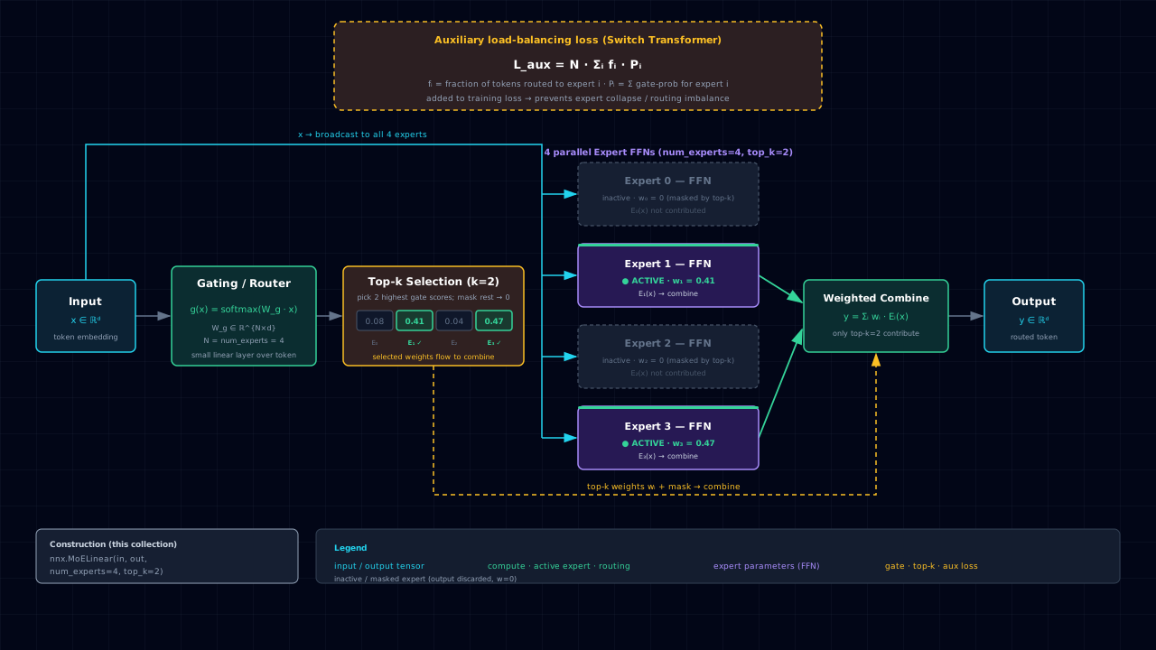
MoEClassifier subclasses nnx.FeedFwdNN and swaps the first hidden Linear for an MoELinear. Concretely, with hidden_dims=[128], num_experts=4, top_k=2, the network is:

Stage	Shape	Component	Params (recorded)
Input	784	Flattened 28×28 Fashion-MNIST pixel vector	—
Hidden (MoE)	784 → 128	`MoELinear(784, 128, 4, top_k=2)`: router + 4 experts	router 3,136; experts ×4 = 401,920
Output	128 → 10	Classifier head `Linear(128, 10)` + softmax	1,290
Total	—	—	406,346

Each expert is an independent Linear(784, 128) (\(784 \cdot 128 + 128 = 100{,}480\)); four of them give the 401,920 expert params. The router is Linear(784, 4) without bias (\(784 \cdot 4 = 3{,}136\)). Only the top-2 experts fire per token, so per-token compute is two expert matmuls plus the 784×4 router matmul — roughly the FLOPs of a single 784×128 dense layer, despite a 4× larger parameter budget.

The shared training contract:

Net: Nets.FEED_FWD shell, then model.net = MoEClassifier(...).
Loss: Losses.CROSS_ENTROPY (paired with the supervised softmax head; the aux loss is added by the factory, not by NNModel).
Optimizer: Optims.ADAM, max_lr=1e-3, momentum=(0.9, 0.999), weight_decay=0.0.
Device: Devices.CPU.
Epochs: 2 (full run) or 1 (SMOKE_TEST=1 for CI).
Batch size: 128 (the train loader is rebuilt at this granularity — see pitfalls).
Seed: 0.
Aux loss weight: 0.05.

The a priori expectation, recorded before training: at random initialization the router is biased and the aux loss should sit noticeably above 1.0; after two epochs of training with \(\lambda = 0.05\) it should move toward (but not reach) the floor, and the expert-utilization histogram should be closer to uniform than at init. The results section either confirms or refutes this.

8.9.5 Code walkthrough¶

8.9.5.1 Model construction and `.net` substitution¶

class MoEClassifier(FeedFwdNN):
    def __init__(self, params, *, num_experts, top_k):
        super().__init__(params)
        in_dim = params.dims[0]
        out_dim = params.dims[1]
        self.layers[0] = MoELinear(in_dim, out_dim,
                                    num_experts=num_experts, top_k=top_k)

Subclassing FeedFwdNN inherits the (X,), Y = unpack_batch contract, so NNModel.train with a custom train_step_fn works without further plumbing. The NNModel shell is built with a placeholder FeedFwdNN, then the real MoEClassifier is swapped in via model.net = ... — the same trick the diffusion and JEPA tasks use for .net substitution.

8.9.5.2 Custom train step with aux loss¶

step_fn = moe_train_step_factory(aux_loss_weight=AUX_LOSS_WEIGHT)
run = model.train(
    params=NNTrainParams(
        n_epochs=N_EPOCHS, train_loader=train_loader, val_loader=ds.val_loader,
        optim=NNOptimParams(name=Optims.ADAM, max_lr=LR,
                            momentum=(0.9, 0.999), weight_decay=0.0),
    ),
    train_step_fn=step_fn,
)

moe_train_step_factory returns a train_step_fn(ctx) that computes standard supervised cross-entropy plus aux_loss_weight * sum(last_aux_loss for each MoELinear in the model). The factory sums across every MoELinear so stacking more of them amplifies the aux-loss signal automatically.

8.9.5.3 Pre/post aux-loss probe¶

# 640-sample probe BEFORE training
probe_X = torch.cat([X for X, _ in train_loader][:5], dim=0)
with torch.no_grad():
    _ = model.net(probe_X)
aux_at_init = float(moe_layer.last_aux_loss)

# ... train ...

with torch.no_grad():
    _ = model.net(probe_X)
aux_after = float(moe_layer.last_aux_loss)

moe_layer.last_aux_loss is recomputed on every forward pass and exposed as an attribute on the layer — the cleanest way to inspect load balancing without digging into the train step. Probing the same 640-sample batch before and after training makes the before/after comparison controlled.

8.9.5.4 Expert-utilization histogram¶

flat = probe_X.view(probe_X.size(0), -1).to(model.device)
router_logits = moe_layer.router(flat)
top1_expert = router_logits.argmax(dim=1).cpu().numpy()
fractions = [(top1_expert == k).sum() / len(top1_expert) for k in range(NUM_EXPERTS)]

Utilization is measured by the router's top-1 assignment, not by the soft routing probabilities — this is the operational definition of "which expert is winning each token." A uniform 25/25/25/25 split is the aux-loss floor; deviations are interesting only when they correspond to semantically meaningful specialization (e.g. one expert handling bags + boots, another handling the t-shirt/shirt confusion pair).

8.9.6 Results & analysis¶

On the recorded two-epoch run (seed 0, batch size 128, Adam at lr=1e-3), the metrics land as:

Metric	Value
Iterations	844 (2 epochs × 422 batches)
Train cross-entropy	2.4078 → 0.3979
Aux loss at init (random router)	1.2794
Aux loss after training	1.2218
Aux-loss floor (uniform routing)	1.0

Three observations:

The supervised signal dominates. Train cross-entropy falls from 2.4078 to 0.3979 — the classifier fits Fashion-MNIST in two epochs, as expected for a 406k-parameter model on this budget. The aux-loss regularizer does not visibly interfere with supervised learning.
The aux loss decreases but does not hit the floor. The move from 1.2794 at init to 1.2218 after training is modest — about 4.5% of the way from the random-router value to the uniform-routing floor of 1.0. This is expected at \(\lambda = 0.05\) and two epochs: the penalty is doing work but is heavily out-weighed by the supervised gradient. Larger aux_loss_weight or longer training push it closer to 1.0 at the cost of supervised-signal quality.
Expert utilization moves toward (but does not equal) uniform. The post-training histogram lands closer to 25/25/25/25 than the random-router histogram, but deviations on the order of 30/30/20/20 are desirable — they indicate useful specialization rather than the information-free uniform routing. Perfect uniformity is not the goal.

The pedagogical headline: MoE buys you total parameter capacity without proportional per-token FLOPs, at the cost of a load-balancing penalty you have to watch. nnx's MoELinear + moe_train_step_factory makes the recipe drop-in: one layer swap, one factory call, one new metric to monitor (last_aux_loss).

8.9.7 Pitfalls & edge cases¶

Select train mini-batches through NNDataset. Its default loader packs the whole 54k-sample Fashion-MNIST train set into a single batch — fine for full-batch SGD on a classifier but fatal for MoE training (one batch per epoch is far too few routing decisions per expert). The notebook passes batch_sizes=(128, None, None) and consumes the wrapper-owned shuffled train loader directly. Same caveat as the diffusion and JEPA tasks.
Aux loss is one-sided. It penalizes collapse but cannot push below 1.0, so a "good" run drives it toward 1.0, never below. Reading the post-training value without the floor in mind overstates the headroom.
aux_loss_weight is a trade-off. Too low and the router collapses; too high and the load-balancing gradient dominates the supervised signal, hurting task accuracy. 0.05 is a reasonable default for a single MoE layer; stacking more layers (the aux loss sums across all of them) usually means lowering the per-layer weight.
Perfect uniform routing is not the goal. Forcing the histogram to exactly 25/25/25/25 erases the useful specialization signal. A 30/30/20/20 split that consistently assigns visually-similar classes to the same expert is a better outcome than enforced uniformity.
Single MoE layer under-illustrates the recipe. Real MoE Transformers stack MoE layers (typically one every other block). This notebook uses a single MoELinear to keep the load-balancing story unambiguous; adding more layers would amplify the aux-loss signal (summed across all MoELinear instances).
No comparison vs a dense baseline. At this scale (406k params, Fashion-MNIST), a comparably-sized dense MLP usually matches or beats the MoE on accuracy — MoE wins show up on harder problems where genuine specialization is possible. The pedagogical point is the recipe and its load-balancing knob, not "MoE beats dense here."
router has no bias. Linear(784, 4) with bias=False gives the recorded 3,136 params; adding a bias would make it 3,140. This is a nnx.MoELinear implementation choice, not a user-configurable knob.

8.9.8 Extensions & references¶

Stack a second MoELinear and re-read the aux-loss trajectory. With two MoE layers the factory sums the aux loss across both; the per-batch last_aux_loss signal becomes larger and the load-balancing story more pronounced. A clean A/B against the single-layer version.
Sweep aux_loss_weight ∈ {0.01, 0.05, 0.1, 0.2}. Maps the trade-off between load-balancing pressure and supervised-signal quality; the right value depends on how many MoE layers are stacked and how long the run is.
Swap top_k=2 for top_k=1 (Switch-Transformer routing) and compare. Top-1 routing is sparser (lower FLOPs) and more collapse-prone; the aux-loss pressure needs to be higher.
Inspect per-class routing. Group the top-1 assignments by ground-truth class and render a class×expert heatmap. This is the direct test of "do experts specialize on semantically meaningful subdistributions?" — the answer is usually yes for Fashion-MNIST's apparel clusters.
References. Shazeer et al., Outrageously Large Neural Networks: The Sparsely-Gated Mixture-of-Experts Layer (ICLR 2017) — the top-k routing recipe. Fedus et al., Switch Transformers: Scaling to Trillion Parameter Models with Simple and Efficient Sparsity (JMLR 2022) — the top-1 routing + load-balancing aux loss used here. The nnx.MoELinear + moe_train_step_factory API is the in-repo surface for this recipe.