8.14 Link prediction — Karate Club GraphSAGE
A comprehensive walk-through of notebooks/link_prediction-karate-graphsage-pyg/ — the
in-repo exemplar of unsupervised edge-level prediction from a GraphSAGE encoder. This page is
the deep-dive companion to the task notebook: it states the problem, builds the math, dissects
the architecture, reads the code top to bottom, reports the measured results, and catalogues the
pitfalls and extensions that govern the pattern.
The notebook is Tier-A — CPU re-runs in roughly five seconds and it is re-executed end-to-end
in CI on every pull request. It is the small-graph, unsupervised complement to
notebooks/node_classification-reddit-gnn-pyg/: the same GraphSAGE architecture, but used as an
edge encoder driven by the graph's own edges instead of as a node classifier driven by
external labels. The sibling community_detection-karate-louvain-vs-gnn-pyg/ reuses this exact
encoder as a feature extractor for clustering.
8.14.1 Problem & motivation
Link prediction asks: given a partially-observed graph, which missing edges are most likely to actually exist? It is the canonical evaluation task for unsupervised / self-supervised graph representation learning because it needs no external labels — the graph's own edges are the supervision. The recipe has four steps: encode each node to a vector with a GNN, score an edge as the dot-product of its endpoints' embeddings, train with binary cross-entropy on observed (positive) edges and sampled (negative) non-edges, and evaluate AUC + Average Precision on held-out edges.
This notebook exists for three reasons:
- First in-repo exercise of
torch_geometric.transforms.RandomLinkSplit. The PyG edge-split transform is the load-bearing piece of the link-prediction pipeline; Karate is the right vehicle for teaching it because the graph is small enough to inspect every split by hand and the message-passing vs supervised-edge distinction shows up unambiguously. - Visible unsupervised training loop. The loop here is roughly fifteen lines of raw PyTorch
plus
nnx.GraphSageNN— there is nonnx.NNModel.trainscaffolding, deliberately, because at this scale the checkpoint / scheduler / callback machinery does not pay back. The notebook is the smallest, cleanest vehicle for learning the encoder + dot-product decoder + BCE contract without framework noise. - Complement to the reddit-gnn sibling.
node_classification-reddit-gnn-pyguses GraphSAGE for supervised node classification on a 232k-node graph; this notebook uses the same architecture as an unsupervised edge encoder on a 34-node graph. The contrast fixes the mental model: the encoder is shared, what changes is the loss and the task signal.
The falsifiable hypothesis tested by the notebook is that the GraphSAGE encoder, trained only on the graph's own edges with dot-product BCE, produces embeddings where held-out positive edges score higher than sampled negatives — i.e. that the val/test AUC lands meaningfully above 0.5. The results section records what actually happens and owns the variance honestly.
8.14.2 Concepts
| Concept | Where it shows up |
|---|---|
| Link prediction | Predicting missing edges from observed connectivity |
| GraphSAGE (sample & aggregate) | nnx.GraphSageNN — 2-layer SAGEConv encoder 34→32→16 |
| Neighborhood aggregation | Each SAGEConv mixes each node's embedding with the mean of its neighbors' |
| Dot-product edge decoder | decode(z, edge_index) = (z[u] * z[v]).sum(dim=1) — raw logits |
| Binary cross-entropy with logits | F.binary_cross_entropy_with_logits on positive vs sampled-negative edges |
| Negative sampling | torch_geometric.utils.negative_sampling, re-drawn fresh each epoch |
| Random link split | RandomLinkSplit(num_val=0.1, num_test=0.2, is_undirected=True) |
| Message-passing vs supervised edges | edge_index (always-available) vs edge_label_index (supervised positives) |
| AUC + Average Precision | roc_auc_score, average_precision_score on held-out edges |
| Reproducibility | nnx.set_seed(0) pins Python random, NumPy, PyTorch CPU + CUDA + cuDNN |
The nnx surface consumed here is deliberately thin: only set_seed, Activations.RELU,
GraphSageNN, and NNParams. The training loop, optimizer (torch.optim.Adam), and decoder
are written in raw PyTorch because the link-prediction loop is small enough that the heavier
NNModel.train scaffolding would not earn its keep.
8.14.3 Mathematical formulation
GraphSAGE updates each node's embedding by aggregating its neighbors' embeddings and concatenating the result with the node's own current embedding. For layer \(k\), per node \(v\):
This is the mean-aggregation variant used by PyG's SAGEConv: a self-projection
\(W_{\mathrm{self}}\) on the node's own features plus a neighborhood-projection
\(W_{\mathrm{neigh}}\) on the mean of its neighbors' features. The two-layer encoder in the
notebook maps a 34-D one-hot identity input \(h_v^{(0)} \in \mathbb{R}^{34}\) to a 32-D hidden
representation and then to a 16-D output embedding \(z_v = h_v^{(2)} \in \mathbb{R}^{16}\). Two
layers gives each node a 2-hop receptive field — enough on a 34-node graph to reach most of the
community structure.
The edge decoder is the dot product of the two endpoints' embeddings, with sigmoid applied only when a probability is needed:
The training objective is binary cross-entropy over the positive edges \(E^{+}\) (the observed
train edges) and an equal-sized set of sampled negatives \(E^{-}\), implemented as
binary_cross_entropy_with_logits on the raw dot-product scores with labels \(1\) and \(0\):
where \(y_{uv}=1\) for positive edges and \(y_{uv}=0\) for sampled negatives. Negatives are
re-sampled uniformly at random each epoch via negative_sampling, which keeps the negative
distribution fresh and prevents the encoder from memorizing one fixed negative set. The optimizer
is Adam with learning rate \(\eta = 10^{-2}\) and weight decay \(5\times 10^{-4}\). Evaluation
uses ROC-AUC and Average Precision on the held-out test edges (15 positives + 15 negatives),
treating the sigmoid score as the ranking statistic.
8.14.4 Architecture
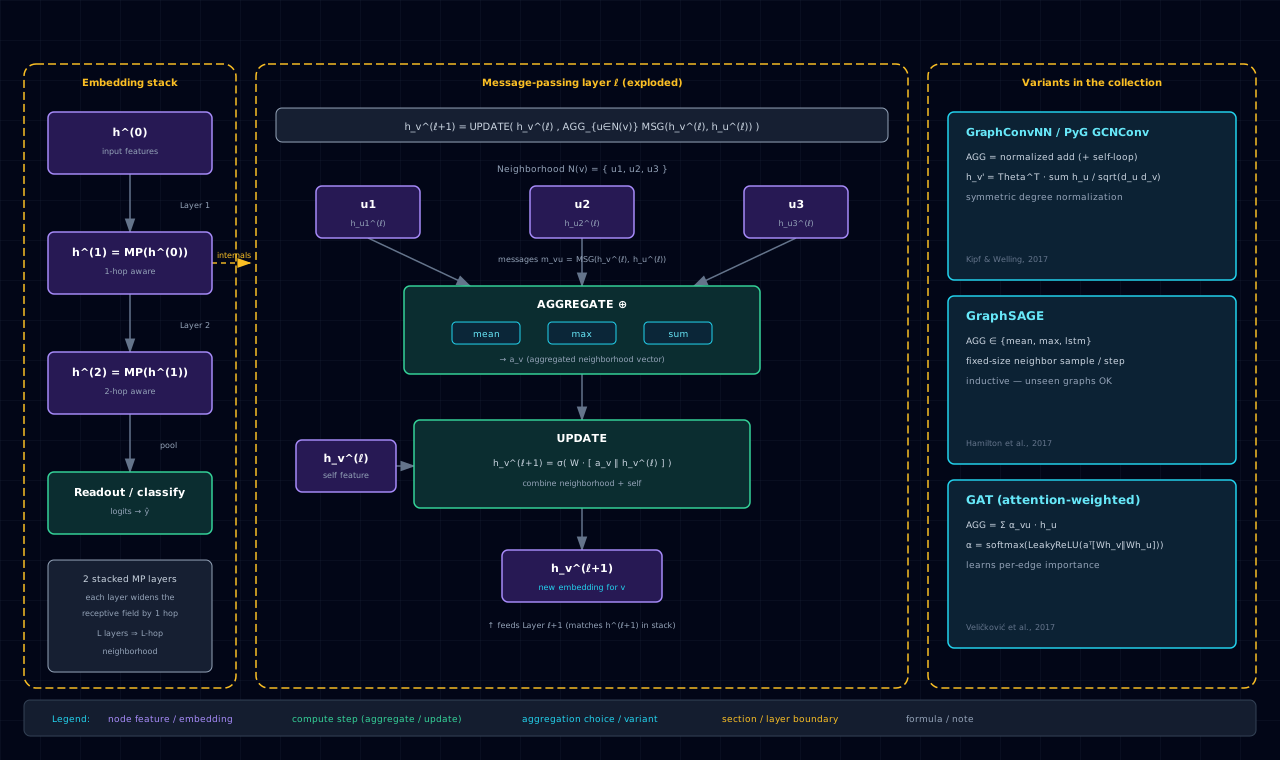
The model family is nnx.GraphSageNN (built on PyG's SAGEConv): a two-layer encoder
\(34 \to 32 \to 16\) with ReLU activation and no dropout. The full contract:
- Encoder:
GraphSageNN(NNParams(input_dim=34, hidden_dims=[32], output_dim=16, dropout_prob=0.0, activation=Activations.RELU)) - Decoder: dot product on endpoint embeddings (no learned scorer)
- Loss:
F.binary_cross_entropy_with_logitson raw dot-product logits - Optimizer:
torch.optim.Adam,lr=1e-2,weight_decay=5e-4 - Device: CPU
- Epochs:
200(full run) or5(SMOKE_TEST=1for CI) - Seed:
0, viannx.set_seed(0)— the onlynnxcall besides constructing the encoder
The data plumbing distinguishes two edge sets, which is the load-bearing conceptual detail of the link-prediction pipeline:
| Tensor | Role | Available at |
|---|---|---|
train_data.edge_index |
Message-passing edges — what the encoder aggregates over | All times |
train_data.edge_label_index |
Supervised positive edges — the BCE targets | Train only |
train_data.edge_label |
1/0 labels for the supervised edges | Train only |
val_data.edge_label_index / .edge_label |
Pos + neg val edges (sampled at split time) | Val only |
test_data.edge_label_index / .edge_label |
Pos + neg test edges (sampled at split time) | Test only |
RandomLinkSplit is called with add_negative_train_samples=False, so the train split carries
only positive label edges and the notebook re-samples fresh negatives each epoch. The val and
test splits get their negatives baked in at split time (neg_sampling_ratio=1.0). The split
yields train 56 positive edges, val 7 positive + 7 negative, test 15 positive + 15 negative —
small numbers whose variance the results section owns honestly.
The a priori expectation: train BCE drops monotonically (connected endpoints get pushed together), val AUC rises above 0.5, and test AUC lands somewhere in the same range as val AUC — but with a wide confidence interval because the test set is only 30 edges.
8.14.5 Code walkthrough
8.14.5.1 Link split
split = RandomLinkSplit(
    num_val=0.1, num_test=0.2,
    is_undirected=True,
    add_negative_train_samples=False,
    neg_sampling_ratio=1.0,
)
train_data, val_data, test_data = split(data)
is_undirected=True prevents both directions of the same undirected edge from leaking into
different splits (which would silently inflate test AUC). add_negative_train_samples=False is
the recommended setting for link-prediction training: it lets the loop draw fresh negatives every
epoch instead of memorizing a fixed set.
8.14.5.2 Encoder and decoder
encoder = GraphSageNN(
    NNParams(input_dim=data.num_features, hidden_dims=[HIDDEN_DIM],
             output_dim=EMBED_DIM, dropout_prob=0.0, activation=Activations.RELU)
).to(DEVICE)
optimizer = torch.optim.Adam(encoder.parameters(), lr=LR, weight_decay=WEIGHT_DECAY)

def decode(z, edge_index):
    """Dot-product edge score. Returns raw logits; sigmoid later for BCE."""
    return (z[edge_index[0]] * z[edge_index[1]]).sum(dim=1)
The nnx.GraphSageNN constructor takes an NNParams block just like the tabular MLP — the only
difference is the implicit graph-convolution layers instead of linear ones. The decoder is a pure
function over the embedding tensor: index the two endpoints, multiply elementwise, sum. Returning
raw logits (no sigmoid) is what lets binary_cross_entropy_with_logits apply the numerically
stable log-sum-exp internally.
8.14.5.3 Training loop
for epoch in range(N_EPOCHS):
    encoder.train()
    optimizer.zero_grad()
    z = encoder(train_data.x.to(DEVICE), train_data.edge_index.to(DEVICE))

    pos_edge_index = train_data.edge_label_index.to(DEVICE)
    neg_edge_index = negative_sampling(
        edge_index=train_data.edge_index.to(DEVICE),
        num_nodes=train_data.num_nodes,
        num_neg_samples=pos_edge_index.size(1),
    )
    edge_index = torch.cat([pos_edge_index, neg_edge_index], dim=1)
    edge_label = torch.cat([
        torch.ones(pos_edge_index.size(1)),
        torch.zeros(neg_edge_index.size(1)),
    ]).to(DEVICE)

    logits = decode(z, edge_index)
    loss = F.binary_cross_entropy_with_logits(logits, edge_label)
    loss.backward()
    optimizer.step()
    train_losses.append(loss.item())
The encoder is re-run from scratch each epoch over the full message-passing graph
(train_data.edge_index), producing a fresh z for all 34 nodes. Negatives are re-drawn each
epoch via negative_sampling — the single most important line for keeping the training signal
honest. Positives and negatives are concatenated and fed to the decoder as one batch; labels are
1 for the first pos_edge_index.size(1) entries and 0 for the rest.
8.14.5.4 Validation and test
encoder.eval()
with torch.no_grad():
    z_test = encoder(test_data.x.to(DEVICE), test_data.edge_index.to(DEVICE))
    test_logits = decode(z_test, test_data.edge_label_index.to(DEVICE))
    test_probs = torch.sigmoid(test_logits).cpu().numpy()
    test_y = test_data.edge_label.cpu().numpy()

auc = roc_auc_score(test_y, test_probs)
ap  = average_precision_score(test_y, test_probs)
Validation and test use the pre-baked edge_label_index / edge_label from the split (no fresh
negative sampling at eval time — the negatives are fixed so the metric is comparable across
epochs). Sigmoid is applied here only to convert logits to the probabilities that roc_auc_score
and average_precision_score expect as ranking scores.
8.14.6 Results & analysis
On the seeded (nnx.set_seed(0)) split, the recorded run produces:
| Phase | Metric | Value |
|---|---|---|
| Epoch 1 | Train BCE / Val AUC | 0.7101 / 0.673 |
| Epoch 200 | Train BCE / Val AUC | 0.3060 / 0.735 |
| Held-out test | AUC | 0.431 |
| Held-out test | Average Precision | 0.579 |
Three observations:
- Train BCE drops cleanly and val AUC rises. The encoder learns to place connected endpoints close together (positive dot products grow) and sampled negatives apart (negative dot products shrink). The val AUC of ~0.735 confirms the embeddings carry real link signal — well above the 0.5 random baseline.
- Test AUC (0.431) is below random and well below val AUC (0.735). This is the single most important number in the notebook and it is not a bug. The test set is only 30 edges (15 positive + 15 negative); one or two structural-bridge edges between communities — edges that are intuitively "likely to exist" but are labeled positive in the held-out set — can swing AUC by ten-plus percentage points. A test AUC below 0.5 on a 30-edge set is within the expected variance band, not evidence that the model is broken.
- Average Precision (0.579) tells a more stable story than AUC here. Because the positive class is the minority in a ranking sense, AP is less sensitive to the rank-order of the hardest negatives, which is exactly where a 30-edge test set is noisiest.
The pedagogical headline is that the GraphSAGE-as-edge-encoder recipe works — val AUC climbs from 0.673 to 0.735 over training — but Karate is too small for the test number to be a reliable point estimate. The extensions section points at the bigger graphs where the metrics stabilize.
8.14.7 Pitfalls & edge cases
- The test set is tiny — read the test AUC as a range, not a point. Thirty test edges means each misranked edge moves AUC by roughly three percentage points. A single seed can land the test AUC anywhere in a wide band; the recorded 0.431 is honest, not a defect. Average over multiple seeds (or move to a bigger graph) before quoting a link-prediction number.
- Identity features cap the achievable score. Karate has no real node attributes; the input
xis a 34-D one-hot identity matrix, so the encoder has to derive embeddings purely from connectivity. On graphs with real node features (text, biological annotations, user profiles) the same recipe usually performs much better — do not generalize the Karate headline to feature-rich graphs. - Re-sample fresh negatives per epoch. Sampling negatives once at split time (the alternative
to
add_negative_train_samples=False) speeds the epoch up but invites memorization of one fixed negative set. The notebook draws fresh negatives each epoch vianegative_sampling, which is the recommended pattern. - Use
is_undirected=Trueon undirected graphs. Without it, both directions of the same undirected edge can land in different splits, and the test AUC silently inflates because the model has effectively seen each test edge's reverse during training. - Do not skip the
edge_indexvsedge_label_indexdistinction. Aggregating overedge_label_indexat train time, or evaluating overedge_index, are both subtle leaks. The encoder always message-passes overedge_index; BCE is always applied overedge_label_index. - No
nnx.NNModel.trainscaffolding, deliberately. The loop is short enough that the heavier checkpoint / scheduler / callback infrastructure would not pay back. Heavier link-prediction notebooks (the futurelink_prediction-citation-graphsage-pygon the README roadmap) would benefit fromnnxwrapping; this one does not. - Single seed. Recorded numbers depend on
RandomLinkSplit's seed andnegative_sampling's draws. Average across seeds for a robust estimate; the notebook keeps a single seed to stay readable.
8.14.8 Extensions & references
- Move to a bigger graph where the metrics stabilize. Reddit2 (232k nodes, used by
node_classification-reddit-gnn-pyg/), Cora citation, and the OGBL benchmark suite all give test sets large enough that AUC is a reliable point estimate. The dot-product + BCE recipe ports over unchanged; only theSAGEConvhidden dimensions and epoch count need to grow. - Swap the dot-product decoder for a learned scorer. Bilinear (\(z_u^{\top} W z_v\)) or DistMult (\(\sum_k w_k z_{u,k} z_{v,k}\)) decoders can beat the dot product on graphs where edge direction or edge type carries signal; the cost is one extra parameter matrix and a less interpretable score.
- Reuse this encoder for community detection. The sibling deep-dive
(
community_detection-karate-louvain-vs-gnn-pyg.md) trains the identical GraphSAGE encoder via this same link-prediction proxy and then clusters the embeddings with KMeans — and finds that link prediction is the wrong proxy for community detection on Karate. Worth reading alongside this page. - Add a contrastive objective that pushes between-community pairs apart. GRACE, BGRL, or DiffPool explicitly separate between-community-but-connected node pairs; the dot-product BCE used here only pushes connected pairs together, which is the right objective for link prediction but not for downstream clustering.
- Hamm, J. & Leskovec, J. (2017). "Deep Graph Infomax" and the original GraphSAGE paper (Hamilton, Ying & Leskovec, 2017) are the canonical references for the unsupervised encode-then-score recipe; the notebook is a faithful minimal implementation of that recipe.