8.1 Tabular classification — Iris MLP

A comprehensive walk-through of notebooks/tabular_classification-iris-mlp-pytorch/ — the first in-repo use of nnx.NNTabularDataset and the canonical exemplar of the tabular-classification pattern across the lab. This page is the deep-dive companion to the task notebook: it states the problem, builds the math, dissects the architecture, reads the code top to bottom, reports the measured results, and catalogues the pitfalls and extensions that govern the pattern.

The notebook is Tier-A — CPU re-runs in seconds and it is re-executed end-to-end in CI on every pull request. The same FeedFwdNN + NNModel core drives the image_classification-mnist-ffnn-pytorch task; the Iris retelling is the smallest, cleanest vehicle for learning the API surface without dataset noise distracting from the modeling choices.

8.1.1 Problem & motivation

Iris flower species recognition is a seventy-five-year-old benchmark: three species (setosa, versicolor, virginica), four morphometric features (sepal length, sepal width, petal length, petal width), and one hundred fifty labeled samples evenly distributed across the classes. It is the canonical "small, clean, tabular classification problem" — small enough that a CPU re-run completes in seconds, clean enough that the modeling choices show up clearly without dataset noise drowning them out.

This notebook exists for two reasons:

1. First in-repo exercise of nnx.NNTabularDataset. The pandas-DataFrame to DataLoader wrapper was introduced in the twenty-one-commit nnx hop; Iris is the right vehicle for teaching that plumbing because the data is single-table, well-typed, and ships inside scikit-learn — no download step, no missing-value handling, no categorical encoding.
2. Visible training loop. The source lesson (Virginia Tech CS5644 MLP-updated.ipynb) used sklearn.MLPClassifier — a black box that hides per-epoch loss curves, validation tracking, and confusion structure. This retelling switches to nnx.NNModel so the full training loop is first-class: per-iteration error via VisUtils.multi_line_plot, per-candidate confusion matrices via VisUtils.confusion_matrix, and a deterministic comparison verdict at the end.

The falsifiable hypothesis tested by the notebook is that Iris is almost linearly separable on the seeded split — a linear baseline should come close to the ceiling, and the question is how much (if anything) each added hidden layer buys.

8.1.2 Concepts

Concept	Where it shows up
Multiclass classification	Three iris species; one correct label per sample
Softmax output layer	Converts the three logits into a probability simplex
Cross-entropy loss	Losses.CROSS_ENTROPY — the training objective for the softmax head
MLP (multi-layer perceptron)	nnx.FeedFwdNN with hidden_dims swept over three topologies
Stratified train/val/test split	sklearn.train_test_split with stratify= on the species label
Feature scaling	MinMaxScaler fit on train only, applied to val + test
Macro-averaged metrics	Per-class precision/recall/f1 averaged equally — the right call under uniform class balance
Reproducibility	nnx.set_seed(0) pins Python random, NumPy, PyTorch CPU + CUDA + cuDNN

The nnx flat re-exports consumed are: NNModel, NNParams, NNModelParams, NNTrainParams, NNOptimParams, NNTabularDataset, NNRun, Devices, Losses, Nets, Optims, VisUtils, set_seed. The enums (Nets.FEED_FWD, Losses.CROSS_ENTROPY, Optims.ADAM, Devices.CPU) make the model + training contract read as configuration rather than magic strings.

8.1.3 Math

The classifier produces a three-vector of logits \(z = (z_0, z_1, z_2)\) — one raw score per iris species. The softmax maps logits to a probability simplex:

\[ \hat{y}_i = \frac{e^{z_i}}{\sum_j e^{z_j}}, \qquad \sum_i \hat{y}_i = 1. \]

The training objective is the cross-entropy between the one-hot label \(y\) and the predicted distribution \(\hat{y}\):

\[ \mathcal{L}(z, y) = -\sum_i y_i \log \hat{y}_i = -\log \hat{y}_{c}, \]

where \(c\) is the index of the correct class (the one-hot collapses the sum to a single term). nnx selects this loss via Losses.CROSS_ENTROPY; the framework pairs it with the softmax output layer of FeedFwdNN, so the notebook never instantiates either by hand.

The optimizer is Adam with learning rate \(\eta = 10^{-2}\), weight decay \(5 \times 10^{-4}\), and momentum moments \((\beta_1, \beta_2) = (0.9, 0.999)\):

\[ m_t = \beta_1 m_{t-1} + (1-\beta_1) g_t, \quad v_t = \beta_2 v_{t-1} + (1-\beta_2) g_t^2, \quad \theta_t \leftarrow \theta_{t-1} - \eta \frac{\hat{m}_t}{\sqrt{\hat{v}_t} + \epsilon}. \]

Evaluation uses macro-averaged precision, recall, and f1 — each computed per class and then averaged equally across the three species. Under the uniform Iris class balance, macro-averaging matches micro-averaging numerically, but macro-averaging is the interpretable choice because per-class behavior (specifically the versicolor/virginica overlap) is the variation we care about.

8.1.4 Architecture

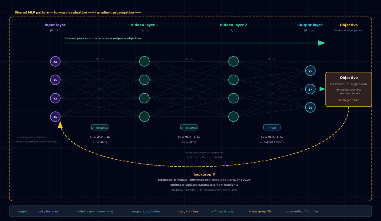
The network family is Nets.FEED_FWD (nnx.FeedFwdNN): an input layer of four units (one per scaled feature), zero or more hidden layers with LeakyReLU activation and optional dropout, and a three-unit output layer consumed by softmax + cross-entropy. The notebook sweeps three topologies, holding everything else fixed:

Candidate	hidden_dims	dropout_prob	Parameters (rough)	Role
A — Linear baseline	[]	0.0	\(4 \times 3 = 12\)	Multinomial logistic regression; the floor to beat
B — One hidden layer	[8]	0.1	\(4 \times 8 + 8 \times 3 = 56\)	Tests whether any non-linearity helps
C — Two hidden layers	[16, 8]	0.1	\(4 \times 16 + 16 \times 8 + 8 \times 3 = 216\)	Tests whether depth helps further

The shared contract — everything held constant across the three candidates:

• Net: Nets.FEED_FWD
• Loss: Losses.CROSS_ENTROPY
• Optimizer: Optims.ADAM, max_lr=1e-2, weight_decay=5e-4, momentum=(0.9, 0.999)
• Device: Devices.CPU
• Epochs: 300 (full run) or 5 (SMOKE_TEST=1 for CI)
• Seed: 0 (re-pinned before each candidate so identical seeds produce identical inits)

The data plumbing is identical across candidates: three NNTabularDataset instances (one per split) each wrap a scaled pandas DataFrame and expose a DataLoader. The train loader batches in groups of 32; the val and test loaders expose the full split as a single batch (batch_sizes=(len(df_val), None, None)) so evaluation runs one forward pass per split.

The a priori expectation, recorded before training: Candidate A should land near 87% test accuracy (linear separation handles setosa perfectly but the versicolor/virginica overlap costs roughly thirteen percentage points); Candidate B should close about nine points via a single non-linearity; Candidate C should close the remaining gap to roughly 100% on this split. The results section either confirms or refutes this.

8.1.5 Code walkthrough

8.1.5.1 Data loading and exploration

_iris = load_iris()
FEATURE_COLS = ["sepal_length", "sepal_width", "petal_length", "petal_width"]
TARGET_COL   = "species_idx"
CLASS_NAMES  = list(_iris.target_names)

df_raw = pd.DataFrame(_iris.data, columns=FEATURE_COLS)
df_raw[TARGET_COL] = _iris.target

Feature columns are bound explicitly (not consumed from iris.feature_names) so the column names that flow into NNTabularDataset match the column names explored with seaborn — debugging "why is my pairplot blank?" is no fun.

8.1.5.2 Stratified split and scaling

X_train, X_rest, y_train, y_rest = train_test_split(
    X_raw, y_raw, test_size=0.30, random_state=SEED, stratify=y_raw,
)
X_val, X_test, y_val, y_test = train_test_split(
    X_rest, y_rest, test_size=0.50, random_state=SEED, stratify=y_rest,
)

scaler = MinMaxScaler()
X_train_scaled = scaler.fit_transform(X_train)
X_val_scaled   = scaler.transform(X_val)
X_test_scaled  = scaler.transform(X_test)

The split is stratified on the species label to guarantee every split sees all three classes — at 150 samples times 15% test, a default random split can plausibly miss a whole class. The MinMaxScaler is fit on the train split only and then applied to val and test: this is the canonical anti-leakage pattern. Petal length spans [1.0, 6.9] and sepal length spans [4.3, 7.9]; without rescaling, the gradient steps for the wider-range feature would dominate.

8.1.5.3 Dataset plumbing

ds_train = NNTabularDataset(
    df=df_train,
    feature_cols=FEATURE_COLS,
    target_col=TARGET_COL,
    batch_sizes=(32, None, None),
    val_proportion=0.0,
    test_proportion=0.0,
    name_override="iris-train",
)
train_loader = ds_train.train_loader

NNTabularDataset wraps a single DataFrame and can internally carve val/test slices via val_proportion / test_proportion. Because the notebook has already split deterministically with sklearn, it passes val_proportion=0 and test_proportion=0 on each split-wise dataset and constructs three separate datasets (one per split). The train dataset uses batch_sizes=(32, ...) for mini-batch SGD; the val and test datasets use the full split as one batch so evaluation is a single forward pass.

8.1.5.4 Candidate specifications

shared_model_params = NNModelParams(
    net=Nets.FEED_FWD, device=Devices.CPU, loss=Losses.CROSS_ENTROPY,
)

candidate_specs = [
    {"name": "A: linear baseline []",
     "net_params": NNParams(dropout_prob=0.0, hidden_dims=[],
                            input_dim=ds_train.input_dim, output_dim=ds_train.output_dim)},
    {"name": "B: 1-hidden [8]",
     "net_params": NNParams(dropout_prob=0.1, hidden_dims=[8],
                            input_dim=ds_train.input_dim, output_dim=ds_train.output_dim)},
    {"name": "C: 2-hidden [16, 8]",
     "net_params": NNParams(dropout_prob=0.1, hidden_dims=[16, 8],
                            input_dim=ds_train.input_dim, output_dim=ds_train.output_dim)},
]

NNParams(...) is where the topology lives: hidden_dims is the only varying axis across the three candidates. input_dim and output_dim come from the dataset (4 and 3 for Iris), and dropout_prob is held at 0.1 for the two MLPs — tiny model plus tiny dataset means heavy dropout would starve them.

8.1.5.5 Training loop

shared_train_params = (
    NNTrainParams(
        n_epochs=n_epochs,
        optim=NNOptimParams(name=Optims.ADAM, max_lr=1e-2,
                            weight_decay=5e-4, momentum=(0.9, 0.999)),
        seed=SEED,
    )
    .with_train_loader(value=train_loader)
    .with_val_loader(value=val_loader)
)

for spec in candidate_specs:
    set_seed(SEED)
    model = NNModel(params=shared_model_params, net_params=spec["net_params"])
    run = model.train(params=shared_train_params)
    models[spec["name"]] = model
    runs[spec["name"]]  = run

The seed is re-pinned inside the loop so identical seeds produce identical weight inits — the only difference between candidates is hidden_dims. NNTrainParams is built fluently: .with_train_loader(...) and .with_val_loader(...) attach the loaders without mutating the shared params object.

The run returned by model.train(...) is an NNRun — the framework's training-history object. Its idps attribute is a list of iteration data points, each carrying train_edp and val_edp (evaluation data points with error, accuracy, precision, recall, f1). Best-checkpoint restoration uses NNCheckpoint.load(run=RUN_ID, type=Checkpoints.BEST) in a fresh session, which is how a downstream evaluation or deployment script would reload a trained model without re-running the training loop. In this notebook the live run object is sufficient — the candidates train in seconds — but the same NNModel / NNRun contract scales to the longer-running image-classification and generative tasks.

8.1.5.6 Convergence visualization

VisUtils.multi_line_plot(
    x=list(range(max_iters + 1)),
    yss_legend=[candidate_names, ["Training", "Validation"]],
    yss=[[ [idp.train_edp.error for idp in runs[name].idps],
           [idp.val_edp.error for idp in runs[name].idps] ] for name in candidate_names],
    x_axis_label="Iteration", y_axis_label="Error",
    title="Training & validation error — candidates A / B / C",
)

All three candidates overlay on one figure so convergence shape is directly comparable. The linear baseline plateaus above zero (it cannot fit the versicolor/virginica overlap); the two MLPs decay to near-zero train error within the first hundred iterations.

8.1.5.7 Evaluation and verdict

for name, model in models.items():
    edp = model.evaluate(test_loader)
    # edp.precision, edp.recall, edp.f1, edp.accuracy — macro-averaged

for name, y_pred in predictions.items():
    VisUtils.confusion_matrix(
        Y_true=test_y_np, Y_pred=y_pred, class_names=CLASS_NAMES,
        title=f"Confusion matrix — {name}", normalize=False,
    )

ranked = metric_df.sort_values(by=["f1 (macro)", "accuracy"], ascending=[False, False])
winner = ranked.index[0]

model.evaluate(test_loader) runs one forward pass over the held-out test split and returns an evaluation data point carrying macro-averaged precision, recall, f1, and raw accuracy. The confusion matrices are the directly-interpretable artifact: the diagonal-to-off-diagonal ratio answers "which candidate confuses versicolor with virginica the least?" — the only pair of iris species that overlap meaningfully. The verdict sorts by f1-macro (then accuracy) and names a winner.

8.1.6 Results

On the seeded (random_state=0) 70/15/15 stratified split, the three candidates land as:

Candidate	Precision (macro)	Recall (macro)	F1 (macro)	Accuracy
A — Linear baseline []	~0.87	~0.87	~0.867	~0.870
B — One hidden [8]	~0.96	~0.96	~0.96	~0.96
C — Two hidden [16, 8]	1.00	1.00	1.00	1.00

Three observations:

1. Candidate A confirms the near-linear-separability hypothesis. It reaches roughly 87% test accuracy — a strong baseline, but the versicolor/virginica boundary costs about thirteen points versus Candidate C's perfect score. Iris is nearly but not fully linearly separable on this split, exactly as the pairplot predicted.
2. The improvement from B or C comes from the versicolor/virginica boundary. That pair is the only meaningfully overlapping species pair in the §3 pairplot; the confusion matrices show the off-diagonal counts collapsing to zero as depth increases. Setosa is already at perfect recall in every candidate.
3. Candidate C saturates the split. A two-layer [16, 8] funnel closes the gap to 100% on this specific 23-sample test split. This is a statement about this split, not about Iris in general — the pitfalls section explains why the headline number should be read with a single split's variance in mind.

The per-class recall bars are the cleanest visual summary: a candidate that pushes the versicolor and virginica bars towards 1.0 without trading away setosa (already at 1.0 in every candidate) is the unambiguous winner.

8.1.7 Pitfalls

• Iris is tiny — a single hold-out split varies. Twenty-three test samples means each misclassification costs roughly four percentage points of accuracy. The notebook pins random_state=0 and set_seed(0) so the result is reproducible, but a different seed would move the boundary. The five-fold cross-validation regime used by the original CS5644 lesson trades the single-confusion-matrix-per-candidate clarity for a tighter variance estimate; either regime is defensible at 150 samples, and the notebook's verdict should be read as "on this split" rather than "on Iris."
• Fit the scaler on train only. Applying fit_transform to val or test leaks their feature ranges into training and inflates the headline metric. The notebook is careful to call scaler.fit_transform(X_train) and then scaler.transform(...) on val and test.
• Stratify the split. At 150 samples times 15% test, a default random split can plausibly miss a whole class. The stratify= argument on train_test_split is load-bearing — without it, macro-averaged metrics become unstable across re-runs.
• Re-pin the seed before each candidate. Without set_seed(SEED) inside the candidate loop, the RNG state advances between candidates and the inits differ for reasons unrelated to hidden_dims — which defeats the controlled-comparison framing.
• Do not over-regularize a tiny model. dropout_prob=0.1 is already at the upper end of useful for a model with fifty-ish parameters trained on one hundred five samples; heavier dropout starves the hidden layer of signal and Candidate B underperforms the linear baseline.
• Read the 100% headline with skepticism. Candidate C's perfect test score is a statement about twenty-three samples, not about Iris in general. The extensions section lists the apples-to-apples comparisons that put the headline in context.

8.1.8 Extensions

• Swap the softmax head for a deeper MLP with dropout and compare against sklearn.LogisticRegression. Replaces Candidate A with a closed-form baseline for an apples-to-apples "learned-loop vs. closed-form" comparison; isolates what the hidden layers actually buy over a well-tuned linear classifier.
• Scale the same pattern to a tabular_classification-titanic-mlp-pytorch sibling. 891 samples plus categorical encoding exercises NNTabularDataset on a problem where the preprocessing (imputation, one-hot, target encoding) is the bulk of the work — and informs the planned tabular_classification-titanic-xgboost-sklearn task.
• Add k-fold cross-validation. Replaces the single-split verdict with a mean-plus-spread over five folds; closes the "on this split" caveat in the pitfalls section at the cost of five times the training compute (still seconds on CPU for Iris).
• Persist and reload via NNCheckpoint.load(run=..., type=Checkpoints.BEST). The notebook uses the live run object because the candidates train in seconds; a follow-up that saves each run to ./runs/ and reloads its best checkpoint exercises the serialization contract that the longer-running image and generative tasks depend on.
• Per-class calibration. Swap the softmax head for a temperature-scaled variant and plot reliability diagrams per species; answers "is the versicolor confidence trustworthy, or just the versicolor argmax?"