8.3 Image classification — MNIST FFNN (NumPy)¶

A comprehensive walk-through of notebooks/image_classification-mnist-ffnn-numpy/ — the from-scratch feed-forward classifier that uses no deep-learning framework. Every gradient is hand-coded; every weight update is a literal W -= lr * dW. This page is the deep-dive companion to the task notebook: it states the problem, derives the math, dissects the layer-by-layer architecture, reads the code top to bottom, reports the measured results, and catalogues the pitfalls and extensions.

The notebook is Tier-A — a full run completes in well under five minutes on CPU and is re-executed end-to-end in CI on every pull request. It is the intentionally standalone sibling of image_classification-mnist-ffnn-pytorch.md: same task, same dataset, but the NumPy variant exists to make the building blocks visible rather than to push accuracy. The nnx library is deliberately not imported here.

8.3.1 Problem & motivation¶

MNIST handwritten-digit recognition is the canonical "first real classifier" benchmark: 60,000 training and 10,000 test 28×28 grayscale images, ten classes (digits zero through nine), roughly class-balanced. It is large enough that a forward pass has real work to do and small enough that a CPU run finishes in minutes.

This notebook exists for one reason, and it is not accuracy:

Every primitive of a feed-forward classifier should be implementable from scratch. Linear layers, parametric ReLU, softmax + cross-entropy, mini-batch SGD with backpropagation — a working classifier whose every gradient and update is visible in this folder's source files.

The falsifiable claim under test is that a network with no autograd and no framework can still learn MNIST. The secondary observation — recorded across two training runs — is how step-size choice (learning rate) governs both convergence speed and validation-loss stability when the architecture is held fixed. The notebook is the sanity counterweight to the PyTorch sibling: it shows what the framework is actually doing for you.

8.3.2 Concepts¶

Concept	Where it shows up
Multiclass classification	Ten digits; one correct label per image
Softmax output layer	`softmax_cross_entropy_layer.py` — converts ten logits into a probability simplex
Cross-entropy loss	`funcs.cross_entropy` — the training objective for the softmax head
Combined softmax + cross-entropy	`SoftmaxCrossEntropyLayer` fuses them so the upstream gradient is the clean `(Y_hat − Y)` — for numerical stability
Parametric ReLU (PReLU)	`relu_layer.py` with `α = 0.01` — leaky nonlinearity on the pre-softmax logits
Fully-connected ("linear") layer	`linear_layer.py` — `Z = X·Wᵀ + b`, the only parametric layer
Backpropagation (chain rule)	`FeedFwdNN.train_and_validate` — forward chains layers, backward iterates in reverse
Mini-batch / full-batch SGD	`Consts.MINI_BATCH_SIZE = 60000` → one batch per epoch = full-batch gradient descent
One-hot encoding	`Utils.one_hot_encode` — labels enter the loss layer as `Y ∈ {0,1}^{n×10}`
Numerical stability	Max-subtraction in softmax; `EPSILON = 1e-30` inside the `log`

There are no nnx symbols in this notebook. The full API surface lives in eight sibling .py files in the task folder: feed_fwd_nn.py, linear_layer.py, relu_layer.py, softmax_cross_entropy_layer.py, funcs.py, consts.py, utils.py, iteration_data_point.py. Reading them in that order is the fastest path to understanding the model.

8.3.3 Mathematical formulation¶

A single image is flattened to \(x \in \mathbb{R}^{784}\) (raw uint8 pixel intensities in \([0, 255]\); no normalization is applied — see §8.3.7). The label is one-hot encoded as \(y \in \{0,1\}^{10}\).

The forward pass composes three layers:

\[ z = x W^{\!\top} + b \qquad (z \in \mathbb{R}^{10}), \]

\[ a = \operatorname{PReLU}_\alpha(z), \qquad \operatorname{PReLU}_\alpha(z_i) = \begin{cases} z_i & z_i > 0 \\ \alpha\, z_i & z_i \leq 0 \end{cases}, \quad \alpha = 0.01, \]

\[ \hat{y} = \operatorname{softmax}(a), \qquad \hat{y}_i = \frac{e^{a_i}}{\sum_j e^{a_j}}. \]

The loss is the mean cross-entropy over the \(n\) samples in the batch, with a tiny \(\varepsilon = 10^{-30}\) added inside the log for numerical stability:

\[ \mathcal{L} = \frac{1}{n}\sum_{k=1}^{n} \sum_{i=0}^{9} -y_{k,i}\, \log\!\bigl(\hat{y}_{k,i} + \varepsilon\bigr) = \frac{1}{n}\sum_{k=1}^{n} -\log\!\bigl(\hat{y}_{k, c_k} + \varepsilon\bigr), \]

where \(c_k\) is the correct class index (the one-hot collapses the inner sum to a single term).

The backward pass applies the chain rule in reverse. The crucial simplification — and the reason SoftmaxCrossEntropyLayer is fused — is that the gradient of the combined softmax-plus-cross-entropy objective with respect to the pre-softmax activations \(a\) is exactly:

\[ \frac{\partial \mathcal{L}}{\partial a} \;=\; \hat{y} - y \;\in\; \mathbb{R}^{n \times 10}. \]

This avoids ever forming the (ill-conditioned) Jacobian of softmax. The PReLU layer multiplies element-wise by its derivative \(\frac{d a_i}{d z_i} = \mathbf{1}[z_i > 0] + \alpha\,\mathbf{1}[z_i \leq 0]\). Finally, for the linear layer with \(X \in \mathbb{R}^{n \times 784}\):

\[ \frac{\partial \mathcal{L}}{\partial W} = \frac{1}{n}\, \frac{\partial \mathcal{L}}{\partial z}^{\!\top} X \quad\in \mathbb{R}^{10 \times 784}, \qquad \frac{\partial \mathcal{L}}{\partial b} = \frac{1}{n} \sum_{k=1}^{n} \frac{\partial \mathcal{L}}{\partial z_k} \quad\in \mathbb{R}^{10}. \]

The update is vanilla SGD with no momentum — learning rate \(\eta\) is the only hyperparameter of the optimizer:

\[ W \leftarrow W - \eta\, \frac{\partial \mathcal{L}}{\partial W}, \qquad b \leftarrow b - \eta\, \frac{\partial \mathcal{L}}{\partial b}. \]

8.3.4 Architecture¶

Feed-forward MLP

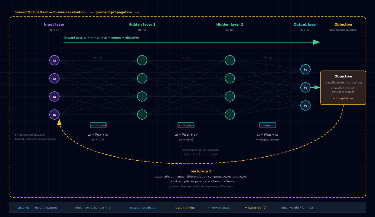
FeedFwdNN composes exactly three layer objects; the full graph is:

X (n×784, raw uint8) ──► LinearLayer(784→10) ──► ReluLayer(PReLU α=0.01)
                                                     │
                                                     ▼
                              SoftmaxCrossEntropyLayer ◄── Y (n×10 one-hot)

Layer	File	Parameters	Role
`L1` Linear	`linear_layer.py`	\(W \in \mathbb{R}^{10\times784}\), \(b \in \mathbb{R}^{10}\) (7850 total)	The only learnable layer
`L2` PReLU	`relu_layer.py`	0 (α is a fixed constant)	Element-wise nonlinearity on the 10 logits
`L3` Softmax+CE	`softmax_cross_entropy_layer.py`	0	Loss + fused gradient

Be precise about what this is and is not: it is a linear classifier with a parametric-ReLU nonlinearity applied to the pre-softmax logits. It is not a multi-layer perceptron in the usual "784 → H → 10 with hidden units" sense — there is no hidden layer wider than the output, and the only weights are the single projection from 784 pixels directly to the 10 class logits. The PReLU lets the model suppress strongly-negative logits towards zero rather than propagating them as large negative scores into the softmax, which is a small amount of expressive power over a bare linear classifier.

Weight initialization. W is drawn from np.random.standard_normal and then L2-normalized as a whole matrix (W / ||W||_F), and similarly b is L2-normalized as a vector. This is not Xavier/He initialization — it bounds the Frobenius norm of the whole weight matrix to 1 but says nothing about per-unit fan-in scaling.

The two training runs share this exact architecture; the only varying axis is the learning rate:

Run	`lr`	`n_epochs`	`mini_batch_size`	Optimizer
`net1`	`0.1` (`Consts.LR`)	`5000` (or `10` under `SMOKE_TEST=1`)	`60000` (= full train set)	vanilla SGD
`net2`	`0.01`	`5000` (or `10` under `SMOKE_TEST=1`)	`60000`	vanilla SGD

Because mini_batch_size equals the entire 60,000-sample training set, each epoch performs exactly one gradient step on the full-batch mean loss — this is full-batch gradient descent, not stochastic mini-batch SGD, despite the parameter name. The full sweep is therefore 5000 iterations; the smoke run exercised in CI is 10.

8.3.5 Code walkthrough¶

8.3.5.1 The linear layer (`linear_layer.py`)¶

def forward(self, X):
    self.X = X
    Z = linear(self.X, self.W, self.b)   # np.matmul(X, W.T) + b
    return Z

def backward(self, dL_dZ):
    n = self.X.shape[0]
    dW = 1./n * dL_dZ.T @ self.X
    db = 1./n * dL_dZ.T.sum(axis=1, keepdims=True).reshape(-1)
    return dW, db

forward caches the input batch (self.X) so backward can compute the weight gradient as the outer-product mean of upstream-gradient × input. This cache is exactly what an autograd framework would record on the tape — here it is a literal attribute assignment. Note the 1/n factor: the gradient is averaged across the batch to match the mean in the loss.

8.3.5.2 The PReLU layer (`relu_layer.py`)¶

def forward(self, Z):
    self.Z = Z
    return parametric_relu(Z, Consts.PARAMETRIC_RELU_ALPHA)   # np.where(Z>0, Z, α*Z)

def backward(self, dL_dA):
    dA_dZ = parametric_relu_prime(self.Z, Consts.PARAMETRIC_RELU_ALPHA)  # np.where(Z>0, 1, α)
    return dL_dA * dA_dZ

The backward pass is the element-wise product of the upstream gradient with the PReLU derivative — the chain rule for an element-wise nonlinearity. The leaky slope α = 0.01 means dead-negative-region gradients are 1% of the positive slope, not strictly zero as in vanilla ReLU.

8.3.5.3 The fused softmax + cross-entropy layer (`softmax_cross_entropy_layer.py`)¶

def forward(self, A, Y):
    self.Y = Y
    Y_hat = softmax(A)            # exp(A - max) / sum, row-wise
    self.Y_hat = Y_hat
    return cross_entropy(Y, Y_hat)

def backward(self):
    return smce_prime(self.Y, self.Y_hat)   # Y_hat - Y

This is the most important fusion in the notebook. Computing softmax and cross-entropy as separate layers would require materializing the softmax's \(10 \times 10\) per-sample Jacobian; fusing them collapses the whole thing to \(\hat{y} - y\). The softmax itself subtracts the per-row max before exponentiating to avoid overflow on the raw [0, 255] inputs (whose initial logits can be large), and the cross-entropy adds EPSILON = 1e-30 inside the log to stay finite when the model is confidently wrong early in training.

8.3.5.4 The training loop (`feed_fwd_nn.py`)¶

for epoch_idx in range(self.n_epochs):
    for mb_idx, I in enumerate(Utils.mini_batchify(self.I_train, self.mini_batch_size)):
        X, Y = self.X_train[I], self.Y_train[I]

        A1 = self.L1.forward(X)
        A2 = self.L2.forward(A1)
        L_train = self.L3.forward(A2, Y)

        dA2 = self.L3.backward()
        dA1 = self.L2.backward(dA2)
        dW, db = self.L1.backward(dA1)

        self.L1.W -= self.lr * dW
        self.L1.b -= self.lr * db

        L_val = self._validate()
        iteration_data.append(IterationDataPoint(...))

This is the whole story. Forward runs L1 → L2 → L3; backward runs L3 → L2 → L1 and yields (dW, db) for the only parametric layer; SGD applies the update by hand. The validation loss is recomputed inside the loop after every train step.

Two subtle points are worth flagging. First, _validate() reuses the same self.L1 / L2 / L3 objects as training rather than constructing fresh ones — this is safe only because validation runs after the training backward pass has already consumed (and thus can no longer be confused by overwriting) the cached self.X / self.Z activations; the source comment calls this out explicitly. Second, with mini_batch_size = 60000, the inner for mb_idx loop body runs exactly once per epoch — one gradient step per epoch.

8.3.5.5 Data plumbing¶

ds_train = thv.datasets.MNIST(root="./data", train=True, download=True, ...)
X_train = ds_train.data.numpy().reshape(-1, 784)            # raw uint8, NOT normalized
Y_train = Utils.one_hot_encode(ds_train.targets.numpy(), C=[0,1,...,9])

torchvision is used only to download and surface the MNIST tensors; the notebook reads ds.data.numpy() directly, bypassing the transform= pipeline entirely. Consequently no ToTensor / Normalize / [0,1] rescaling happens — the model trains on raw 0–255 integers. The labels are one-hot encoded once upfront and reused for every batch.

8.3.5.6 The two-run comparison¶

The same FeedFwdNN class is instantiated twice — net1 at lr=0.1 (Consts.LR) and net2 at lr=0.01 — and Utils.two_line_plot overlays training vs. validation loss for each. The notebook does not track accuracy or per-class metrics; IterationDataPoint carries only training_loss, validation_loss, and the iteration/epoch/minibatch indices.

8.3.6 Results & analysis¶

The committed notebook outputs reflect a SMOKE_TEST=1 run (10 epochs = 10 full-batch gradient steps, since the batch size equals the training set). At that early stage the two runs land at:

Run	`lr`	Best validation loss (10 steps)
`net1`	`0.1`	≈ 47.13
`net2`	`0.01`	≈ 35.17

Two observations:

Both losses are large in absolute terms. A random 10-way classifier sits at \(\log 10 \approx 2.3\) nats of cross-entropy; losses in the tens mean the model is confidently wrong on much of the validation set after only ten updates. The cause is the raw [0, 255] inputs combined with the huge initial logits: with L2-normalized W but 784-dimensional inputs each in the hundreds, the pre-softmax logits can reach magnitudes where softmax saturates hard, and a wrong-but-confident prediction contributes nearly \(-\log(10^{-30}) \approx 69\) to the loss. This is the visible cost of skipping input normalization — see §8.3.7.
The smaller learning rate is lower-loss at this early stage. With unnormalized inputs the per-step gradients are large; lr=0.1 overshoots and oscillates, while lr=0.01 takes smaller, steadier steps that monotonically reduce validation loss over the first ten iterations. The notebook's headline observation — that step size governs stability more than speed on this raw-input setup — is exactly what the curves show.

The full 5000-epoch run converges substantially further (the smoke run is what is CI-affordable); the value of the committed numbers is qualitative (the lr comparison), not as a final-accuracy headline. The notebook deliberately does not report accuracy, confusion structure, or per-class metrics — those are the job of the PyTorch sibling.

8.3.7 Pitfalls & edge cases¶

Inputs are not normalized. X_train / X_val come straight from ds.data.numpy() in raw [0, 255]. The torchvision transform= pipeline is constructed but bypassed. The result is large initial logits, saturating softmax, large early losses, and a learning rate that has to absorb the input-scale variation. Rescaling to [0, 1] (divide by 255) or applying the standard MNIST normalization ((x − 0.1307) / 0.3081) would dramatically improve conditioning — and is what the PyTorch sibling does. This is the single biggest "why is the loss so high?" surprise for a reader.
No seeds are set. LinearLayer.__init__ draws from unseeded np.random.standard_normal, and the train-index sampling uses unseeded np.random.randint. Two consecutive runs of the notebook will diverge; the recorded smoke numbers are illustrative, not reproducible. Add np.random.seed(0) early in the setup cell to fix this.
It is full-batch gradient descent, not mini-batch SGD. Consts.MINI_BATCH_SIZE = 60000 equals the entire training set, so the inner for mb_idx loop runs once per epoch and n_epochs literally equals the iteration count. Reducing MINI_BATCH_SIZE (e.g. to 64) is the easiest way to get true stochastic noise and faster per-epoch wall-clock progress.
MINI_BATCH_SIZE = 60000 is also the validation batch. _validate iterates Utils.mini_batchify(self.I_val, self.mini_batch_size), so on the 10,000-image val set this is also a single batch — fine here, but if you cut the constant, validation also changes character.
The "two depths" framing in the README is inaccurate. The actual notebook varies the learning rate across the two runs, not the architecture; both networks are the same single-layer 784 → 10 + PReLU model. Read the source, not the prose, when in doubt.
Numerical precision differs from the PyTorch sibling. Different default floats and accumulation order mean bitwise-different losses and predictions even on identical inputs and inits. This is expected, not a bug.
The L2-normalized init is not Xavier/He. W / ||W||_F bounds the whole-matrix norm to 1 but does not scale by fan-in, so the per-logit activation variance is not controlled. For a single-layer model this is survivable; copying the scheme into a deeper hand-built network would mis-condition it.
Validation reuses the training layer objects. Safe only because the training backward pass has already consumed the cached activations before _validate() is called. If you refactor the loop ordering (e.g. validate before backward), this aliasing will silently corrupt training. The source comment flags this; respect it.

8.3.8 Extensions & references¶

Compare against the PyTorch sibling — image_classification-mnist-ffnn-pytorch.md. Same task and dataset, but the sibling runs an 18-run architecture sweep through the nnx toolkit, normalizes inputs (mean=0.1307, std=0.3081), uses Adam + a ReduceLROnPlateau scheduler, and reaches a ~1.6% validation error. The side-by-side is the clearest illustration of what hand-coding buys (visibility) versus costs (conditioning, optimizer, sweep bandwidth).
Normalize the inputs. Replace ds.data.numpy() with ds.data.float().div(255) (or the full MNIST-standardize transform) and re-run; the loss curve should drop from the tens to well under one within the same ten iterations, and the two-lr comparison becomes a clean convergence-speed story rather than an overshoot story.
Add a hidden layer. Promote the architecture to 784 → H → 10 by inserting a second LinearLayer + ReluLayer pair; this is the smallest change that turns the model into a "real" MLP and is the obvious next teaching step before the convolutional variant the README mentions.
Swap vanilla SGD for momentum or Adam — by hand. The README lists this as future work. Implementing momentum (\(v_t = \mu v_{t-1} + g_t\)) or Adam's bias-corrected moments in the same explicit W -= ... style demystifies what optimizers do and is a natural follow-up exercise.
Track accuracy and per-class metrics. IterationDataPoint currently records losses only. Adding training_accuracy / validation_accuracy fields (computed from np.argmax(Y_hat, axis=1) vs. Utils.one_hot_decode) brings the notebook to parity with the sibling's evaluation surface and makes the lr comparison interpretable as "accuracy over time," not just loss.
Add a tiny convolutional layer (ConvLayer). The README's stated future work — a hand-coded conv layer in the same explicit style — would extend the "every primitive visible" thesis past dense layers and is the natural lead-in to a LeNet-style MNIST variant.