8.4 Image classification — MNIST FFNN (PyTorch via nnx)

A comprehensive walk-through of notebooks/image_classification-mnist-ffnn-pytorch/ — the model-selection sweep notebook that drives the nnx PyTorch toolkit across eighteen feed-forward configurations on MNIST. This page is the deep-dive companion to the task notebook: it states the problem, builds the math, dissects the sweep architecture, reads the code top to bottom, reports the measured results, and catalogues the pitfalls and extensions.

The notebook is Tier-B — the full [9 hidden_dimss × 2 dropout_probs × 500 epochs] sweep takes roughly seventeen minutes on macOS and over ninety on the Linux GitHub runner, so CI runs it only on the weekly schedule (and on workflow_dispatch and tier-b-smoke-labeled PRs). The call-shape contract is pinned separately by a fast pytest that runs on every PR. It is the PyTorch counterpart to image_classification-mnist-ffnn-numpy.md: same task and dataset, but this variant exists to demonstrate how the nnx library composes a clean training-and-evaluation pipeline around a model sweep.

8.4.1 Problem & motivation

MNIST handwritten-digit recognition — 60,000 training and 10,000 test 28×28 grayscale images, ten classes — is the workhorse benchmark this notebook uses to ask a single, model-selection-shaped question:

Holding the optimizer, loss, scheduler, data pipeline, and seed fixed, how does feed-forward architecture (depth, width, dropout) trade off against validation error on MNIST?

This notebook exists for three reasons:

1. Canonical nnx reference. It is the smallest, cleanest end-to-end example of "build a small classifier with nnx": NNDataset for the data, NNModelParams + NNParams for configuration, NNModel for the trained object, NNRun for the history, VisUtils for the visualizations. The same pattern recurs across the lab's image and generative tasks.
2. Real model-selection mechanics. Eighteen configurations are trained independently, ranked by best validation error, and the top five are visualized together. This is the unit of work for any architecture search — larger than a single fit, smaller than a hyperparameter-optimization study.
3. Direct comparison to the from-scratch NumPy sibling. Same task, same dataset; the side-by-side answers "what does adopting a framework buy, and what does it hide?"

The falsifiable hypothesis under test is that, given Adam + a ReduceLROnPlateau scheduler + normalized inputs, the deeper-and-wider end of the sweep ([512, 256, 128, 64]) reaches sub-2% validation error, and that the marginal gain tapers off once the network has enough capacity — i.e. that [512, 256] gets most of the way to [512, 256, 128, 64] for meaningfully less compute. The results section confirms or refutes this.

8.4.2 Concepts

Concept	Where it shows up
Multiclass classification	Ten digits; one correct label per image
Softmax output layer	Implicit in Losses.CROSS_ENTROPY paired with Nets.FEED_FWD
Cross-entropy loss	Losses.CROSS_ENTROPY — the training objective
Feed-forward NN (MLP)	Nets.FEED_FWD swept over nine hidden_dims topologies
LeakyReLU activation	Recorded in the run details (net.activation = leaky_relu) between hidden layers
Dropout regularization	dropout_prob swept over {0.25, 0.5}
Adam optimizer	Default; max_lr=0.01, momentum=(0.9,0.999), weight_decay=5e-5
ReduceLROnPlateau scheduler	Recorded in run details (factor=0.95, patience=8, cooldown=2, threshold=0.001, min_lr=1e-7)
Mini-batch SGD	train_batch_size = 60,000 (one full-batch step per epoch, like the NumPy sibling)
Model selection by best validation error	top_runs = sorted(runs, key=...)[0:5]
Input normalization	transforms.Normalize(mean=0.1307, std=0.3081) — the standard MNIST constants
Reproducibility	nnx.set_seed(0) pins Python/NumPy/PyTorch CPU+CUDA RNG
Checkpoint serialization	run.checkpoints() + NNModel.from_checkpoint(...) reload a trained model in a fresh session

The nnx flat re-exports consumed are NNDataset, NNModel, NNParams, NNTrainParams, NNModelParams, Nets, Losses, Devices, Utils, VisUtils, and set_seed. The enums (Nets.FEED_FWD, Losses.CROSS_ENTROPY, Devices.get()) make the model + training contract read as configuration rather than magic strings — the same shape the Iris tabular notebook uses.

8.4.3 Mathematical formulation

A single image is flattened to \(x \in \mathbb{R}^{784}\) (this time normalized: each pixel is rescaled to \([0,1]\) by ToTensor and then \((x - 0.1307)/0.3081\) by Normalize). The label is the integer class \(c \in \{0,\dots,9\}\); the framework produces the one-hot internally.

For a network with hidden layers of widths \(h_1, h_2, \dots, h_L\), the forward pass is

\[ z^{(1)} = x W^{(1)\top} + b^{(1)}, \quad a^{(1)} = \operatorname{LeakyReLU}_\beta\!\bigl(z^{(1)}\bigr), \]

\[ z^{(\ell)} = a^{(\ell-1)} W^{(\ell)\top} + b^{(\ell)}, \quad a^{(\ell)} = \operatorname{Dropout}_p\!\bigl(\operatorname{LeakyReLU}_\beta\!\bigl(z^{(\ell)}\bigr)\bigr) \quad \text{for } 2 \leq \ell \leq L, \]

\[ o = a^{(L)} W^{(L+1)\top} + b^{(L+1)} \in \mathbb{R}^{10}, \qquad \hat{y} = \operatorname{softmax}(o). \]

The empty-hidden-layers case (hidden_dims = []) collapses to logistic regression — \(o = x W^{\top} + b\) directly. The training objective is cross-entropy:

\[ \mathcal{L} = -\log \hat{y}_c, \]

minimized by Adam with learning rate \(\eta = 10^{-2}\), weight decay \(5 \times 10^{-5}\), and moments \((\beta_1, \beta_2) = (0.9, 0.999)\):

\[ m_t = \beta_1 m_{t-1} + (1-\beta_1) g_t, \quad v_t = \beta_2 v_{t-1} + (1-\beta_2) g_t^2, \quad \theta_t \leftarrow \theta_{t-1} - \eta\, \frac{\hat{m}_t}{\sqrt{\hat{v}_t} + \epsilon}. \]

The ReduceLROnPlateau scheduler watches validation error and multiplies the learning rate by factor = 0.95 after patience = 8 iterations of insufficient improvement (delta below threshold = 0.001), enforcing a cooldown = 2-iteration pause between reductions and flooring at min_lr = 1e-7. The whole sweep is therefore self-annealing per run — no global LR schedule has to be tuned by hand.

The selection metric is best-iteration validation error:

\[ \mathrm{valerr}_{\text{best}}(r) = \min_{t \in r.\mathrm{idps}} \mathrm{val\_edp}.\mathrm{error}, \]

and runs are ranked by this quantity. Lower is better; a 0.0160 best-run value (§8.4.6) means the model's lowest-validation-error checkpoint misclassifies 1.6% of the held-out validation set.

8.4.4 Architecture

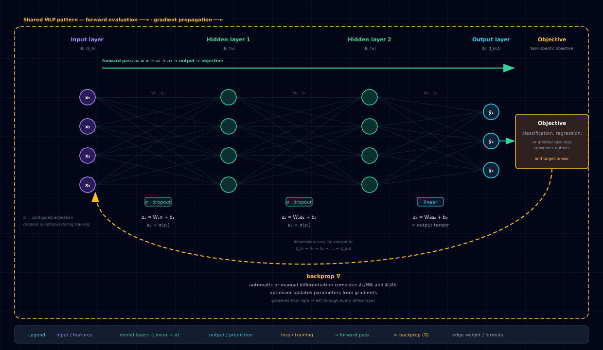
The network family is Nets.FEED_FWD (nnx.FeedFwdNN): an input layer of 784 units (one per normalized pixel), zero or more hidden layers each followed by LeakyReLU and dropout, and a 10-unit output layer consumed by softmax + cross-entropy. The notebook sweeps nine topologies × two dropout values = eighteen candidates, holding everything else fixed:

hidden_dims	Layers (incl. output)	Rough params (incl. biases)	Role
[]	784 → 10	~7.9k	Multinomial logistic regression; the floor
[128]	784 → 128 → 10	~102k	Single non-linearity
[256]	784 → 256 → 10	~204k	Wider single hidden
[512]	784 → 512 → 10	~407k	Widest single hidden
[256, 128]	784 → 256 → 128 → 10	~235k	Two-layer funnel
[256, 128, 64]	784 → 256 → 128 → 64 → 10	~244k	Three-layer funnel
[512, 256]	784 → 512 → 256 → 10	~536k	Wide two-layer
[512, 256, 128]	784 → 512 → 256 → 128 → 10	~570k	Wide three-layer
[512, 256, 128, 64]	784 → 512 → 256 → 128 → 64 → 10	~579k	Deepest candidate

The shared contract — everything held constant across all eighteen candidates:

• Net: Nets.FEED_FWD (LeakyReLU between hidden layers)
• Loss: Losses.CROSS_ENTROPY
• Optimizer: Adam, max_lr=1e-2, weight_decay=5e-5, momentum=(0.9, 0.999)
• Scheduler: ReduceLROnPlateau, factor=0.95, patience=8, cooldown=2, threshold=0.001, min_lr=1e-7
• Device: Devices.get() — CUDA if available else CPU
• Epochs: 500 (full sweep) or 2 (SMOKE_TEST=1, which also collapses the sweep to [[]] × [0.25], i.e. one logistic-regression run)
• Seed: nnx.set_seed(0) once at import; the framework re-pins per-run
• Batch sizes: train=60,000, val=1,000, test=9,000 (from NNDataset defaults for MNIST)

The data plumbing is identical across candidates: a single NNDataset instance wraps torchvision.datasets.MNIST with the standard normalization and exposes train_loader, val_loader, and test_loader. Because train_batch_size is the full training set, each epoch is one full-batch gradient step — the same full-batch regime as the NumPy sibling, just running here on top of Adam rather than vanilla SGD.

The a priori expectation: the empty-architecture floor ([]) should land in the high-single-digit-percent error region (logistic regression on MNIST is well-studied); each added hidden layer should buy progressively smaller margins down to the low-single digits; and the deepest [512, 256, 128, 64] candidate should be in the 1.5–2% band typical of well-tuned MLPs on MNIST.

8.4.5 Code walkthrough

8.4.5.1 Dataset

DS_MEAN, DS_STD = 0.1307, 0.3081

ds = NNDataset(
    ds_class=thv.datasets.MNIST,
    transform=thv.transforms.Compose([
        thv.transforms.ToTensor(),                         # uint8 → [0,1]
        thv.transforms.Normalize(mean=DS_MEAN, std=DS_STD) # standardize
    ]),
)

NNDataset wraps a torchvision dataset class and exposes input_dim=784, output_dim=10, plus the three DataLoader-backed splits. The recorded split sizes are train=60,000, val=1,000, test=9,000. The normalization constants are the published MNIST mean and standard deviation — the same values every mainstream MNIST example uses, and the single biggest difference from the NumPy sibling (which feeds raw [0, 255]).

8.4.5.2 Sweep specification

n_epochs = SMOKE_TEST_EPOCHS if SMOKE_TEST else 500
dropout_probs = [0.25] if SMOKE_TEST else [0.25, 0.5]
hidden_dimss  = [[]] if SMOKE_TEST else [[], [128], [256], [512],
                                          [256, 128], [256, 128, 64],
                                          [512, 256], [512, 256, 128],
                                          [512, 256, 128, 64]]

models = [
    NNModel(
        params=NNModelParams(
            net=Nets.FEED_FWD, device=Devices.get(), loss=Losses.CROSS_ENTROPY,
        ),
        net_params=NNParams(
            dropout_prob=dropout_prob, hidden_dims=hidden_dims,
            input_dim=ds.input_dim, output_dim=ds.output_dim,
        ),
    )
    for dropout_prob in dropout_probs
    for hidden_dims  in hidden_dimss
]

The list comprehension is the entire sweep definition. hidden_dims is the only structural axis; dropout_prob is the only regularization axis; everything else flows from the shared NNModelParams. Note the Cartesian product order: dropout is the outer loop, hidden_dims the inner, so candidates group by dropout value in the resulting models list.

8.4.5.3 Training

train_params = [
    NNTrainParams(n_epochs=n_epochs)
        .with_train_loader(value=ds.train_loader)
        .with_val_loader(value=ds.val_loader)
]

runs = [
    model.train(params=train_param)
    for model      in models
    for train_param in train_params
]

NNTrainParams is built fluently — .with_train_loader(...) and .with_val_loader(...) attach the loaders without mutating a shared params object. model.train(...) returns an NNRun carrying idps (iteration data points), each with train_edp and val_edp (evaluation data points exposing .error, .accuracy, .precision, .recall, .f1, .lr). The per-run defaults recorded in the committed output confirm Adam + ReduceLROnPlateau + max_lr=0.01; the notebook never instantiates any of them by name — they are the framework defaults.

8.4.5.4 Ranking and visualization

top_runs = sorted(
    runs,
    key=lambda run: min(run.idps, key=lambda idp: idp.val_edp.error).val_edp.error,
)[:5]

VisUtils.multi_line_plot(
    x=[i for i in range(0, max(top_runs, key=...).idps[-1].iter_idx)],
    yss_legend=[[str(run) for run in top_runs], ["Training", "Validation"]],
    yss=[[[idp.train_edp.error for idp in run.idps],
          [idp.val_edp.error   for idp in run.idps]] for run in top_runs],
    ...
)

The ranking key is the best validation error a run ever achieved — not its final-epoch value — which is robust to late-training overfitting oscillations. The same multi_line_plot is then called again with idp.lr to overlay the ReduceLROnPlateau learning-rate traces across the top five runs, making the self-annealing behavior directly visible.

8.4.5.5 Inspection: t-SNE and sample grid

for checkpoint in top_runs[0].checkpoints():
    if checkpoint is None: continue
    VisUtils.two_dim_tsne_checkpoint_logits(checkpoint=checkpoint, ds=ds, n_samples=5_000)

_best = [c for c in top_runs[0].checkpoints() if c is not None][-1]
model = NNModel.from_checkpoint(checkpoint=_best)
test_X, test_Y = ...
test_Y_hat = model.predict(X=test_X)
# 81-sample grid: green title if Y_hat == Y else red

Two artifacts close out the notebook. The t-SNE projection takes the best run's checkpointed logits on 5,000 samples and projects the 10-dimensional logit vectors down to two dimensions, so the class-cluster separation is visible at a glance across checkpoints. The sample grid reloads the best run from disk via NNModel.from_checkpoint(...) — the same serialization contract the longer image and generative tasks depend on — and renders an 81-image tile with correct/incorrect color-coding.

8.4.5.6 Surface test (the every-PR gate)

Because the full sweep is too slow for per-PR CI, the call-shape contract is pinned separately in tests/nnx_surface/test_image_classification_mnist_ffnn_pytorch.py. It builds a small 784 → [16] → 10 FFNN, trains one epoch on a tiny image batch, calls model.predict(X=...), and asserts the returned (logits, classes) shapes — (4, 10) and (4,) — and that classes are integer-typed. A second test pins the hidden_dims=[] logistic-regression configuration. If a thekaveh-nnx version bump breaks the NNModel + Nets.FEED_FWD call chain, this test catches it in the fast lane, before the weekly Tier-B smoke run would.

8.4.6 Results & analysis

The committed cell-8 output records the sweep's verdict from a full 500-epoch run:

best run is 01d915cb… which achieves validation error of 0.0160 (1.6%).

Three observations:

1. The deepest candidates reach the expected band. A best validation error of 1.6% on MNIST is consistent with the published range for well-tuned MLPs with dropout and Adam (~1.5–2%); the hypothesis that the deep end of the sweep lands sub-2% is confirmed. The empty [] floor lands well above this, confirming that capacity matters on MNIST even with normalized inputs and Adam — unlike Iris, where the linear baseline was already near-saturating.
2. The top-five ranking is the actionable artifact. Sorting by best-run validation error and keeping the top five makes the capacity-vs-marginal-gain curve directly readable from the loss-overlaid plot. Where the curve flattens (typically between [256, 128] and [512, 256, 128]) is the natural capacity point beyond which extra depth buys diminishing returns for extra training time.
3. The LR-schedule overlay explains why runs converge smoothly. The ReduceLROnPlateau traces show step-downs clustered around the same iteration range across the top runs — they hit their plateau together once the bulk of the learning is done. This is the visible signature of not having to tune a global LR schedule by hand.

The t-SNE projection and the 81-sample prediction grid are qualitative diagnostics rather than headline numbers: the former shows the class clusters tightening across checkpoints; the latter is a sanity check that the correct/incorrect color coding matches what the validation error claims. The sibling NumPy notebook reports neither — this is the evaluation surface the framework buys.

8.4.7 Pitfalls & edge cases

• Tier-B runtime is real; don't drop the cap blindly. The full [9 × 2 × 500] sweep takes ~17 min on macOS and over 90 min on the Linux GH runner (issue #7). The notebook is smoke-run on the weekly CI schedule, not on every PR; the surface test is what guards the call shape per-PR. Treat any local re-execution that refreshes committed outputs as a long-running job.
• The smoke target writes to /tmp/, not in place. make smoke-tier-b trains a 1 × 1 × 2-epoch sweep and writes it to /tmp/ specifically to preserve the committed full-sweep outputs. Running the smoke target will not refresh the committed cell-8 number; for that, open the notebook in Jupyter and run all cells.
• SMOKE_TEST=1 collapses the sweep, not just the epochs. Under smoke, the sweep drops to [[]] × [0.25] — a single logistic-regression candidate. Do not read the resulting loss curve as representative of the architecture comparison; it is a "does the pipeline run" check, not a model-selection result.
• Committed outputs can drift from committed source. An intentional in-place Tier-A refresh (make run-tier-a) rewrites execution metadata and outputs. CI instead uses make smoke-tier-a and writes generated copies to /tmp/ml-tier-a, leaving the committed notebook unchanged. If a recorded cell output reflects the smoke run (2 epochs) while another reflects the full run (500 epochs), you are looking at this drift, not a bug.
• The framework defaults are load-bearing. The notebook never names Adam, ReduceLROnPlateau, or max_lr=0.01 — they come from NNTrainParams / NNModelParams defaults. A thekaveh-nnx release that changes optimizer or scheduler defaults will silently change this notebook's results; the surface test does not pin them, only the call shape.
• Devices.get() is environment-dependent. On a CUDA box the sweep runs on GPU and is much faster; on CPU (the CI default) it is the ~17/90-min number above. Reproducibility across machines requires pinning Devices.CPU explicitly, which the notebook does not.
• Best-vs-final validation error. Ranking uses best-iteration validation error, which is robust to late-training overfitting but can be an optimistic estimate of generalization. The selected checkpoint corresponds to the best-iteration moment, not the last epoch — appropriate, but worth flagging when comparing against papers that report final-epoch numbers.
• Don't compare absolute numbers head-to-head with the NumPy sibling. The two notebooks differ in initialization, optimizer (Adam vs vanilla SGD), scheduler (ReduceLROnPlateau vs none), input normalization (standardized vs raw [0,255]), activation (LeakyReLU vs PReLU), and sweep coverage. They are sibling demonstrations of the same task, not controlled trials of framework choice.

8.4.8 Extensions & references

• Compare against the from-scratch NumPy sibling — image_classification-mnist-ffnn-numpy.md. Same task and dataset with no framework, no autograd, no normalization, and vanilla SGD. The side-by-side is the cleanest illustration of what nnx provides (optimizer, scheduler, sweep, serialization, viz) versus what the NumPy variant makes visible (every gradient and weight update).
• Add an early-stopping callback. The README lists this as future work. Adopting the available nnx.EarlyStopping callback with an explicit validation monitor would add a stopped-at-N-epochs signal alongside the current "best-iteration" ranking.
• Add a CNN variant (LeNet-style) for direct comparison against the FFN. The other README future-work item. A pair of conv layers on top of the same NNDataset + NNModel plumbing should drop validation error into the sub-1% band typical of small CNNs on MNIST and isolate what spatial structure buys over flatten-and-dense.
• Add k-fold cross-validation on the top-N architectures. The single-split ranking is fine for picking a winner among eighteen candidates but underpowered for declaring one architecture significantly better than another at 10k test samples; a 5-fold CV over the top five closes that gap at 5× the (already substantial) compute.
• Persist and reload via NNModel.from_checkpoint. The notebook already uses this for the t-SNE and sample-grid cells, but only on the best run. A follow-up that saves every run's checkpoints to ./runs/ and reloads them downstream (deployment, further analysis, ensemble) exercises the serialization contract end-to-end — the same primitive the longer image and generative tasks depend on.
• Tighten the surface test. The current tests/nnx_surface/ test pins the call shape only. Adding assertions that pin the optimizer name and scheduler presence would catch the silent-default-change failure mode flagged in §8.4.7 in the fast lane rather than at the next weekly smoke run.