8.20 Dimensionality reduction — Iris autoencoder¶
A comprehensive walk-through of notebooks/dim_reduction-iris-autoencoder-pytorch/ — the
canonical demo of two architectural tricks: (1) a FeedFwdNN(input_dim == output_dim,
hidden_dims=[...]) is structurally an autoencoder with no new nn.Module subclass and no
explicit encoder/decoder split; (2) the train_step_fn hook on nnx.NNModel.train lets the
notebook swap in a reconstruction objective (MSE(net(X), X)) while the framework still owns
the scheduler, the val loop, and the checkpoint cadence. This is the first in-repo demo of
train_step_fn outside the transformer LM task.
The notebook is Tier-A — CPU re-runs in ~18 seconds and it is re-executed end-to-end in CI
on every pull request. The comparison is linear PCA (the textbook variance-maximizing baseline)
versus two autoencoder topologies (shallow [2]-bottleneck and symmetric [3, 2, 3]), with
species-separation quality quantified by a held-out linear-probe accuracy on the recovered
2-D latent.
The falsifiable hypothesis tested by the notebook is that a non-linear autoencoder can match or exceed PCA on species separation for iris — but that the deeper autoencoder's extra capacity overfits the reconstruction objective on 150 samples and loses species separation in the bottleneck. The results section either confirms or refutes this.
8.20.1 Problem & motivation¶
Iris has four numeric features (sepal length, sepal width, petal length, petal width) and three species (setosa, versicolor, virginica). Plotting 4-D points directly is impractical, so the standard move is to project to 2-D for visualization. PCA is the linear textbook answer: it picks the two directions of maximum variance. A non-linear autoencoder is the natural next step — same 2-D latent surface, but learned via reconstruction MSE instead of variance-maximizing eigenvectors. The interesting comparison is which one separates the three species more cleanly in the 2-D plane.
This notebook exists for three reasons:
- First
train_step_fndemo outside the LM task. The default supervised forward →loss_fn(net(X), Y)→ backward path doesn't fit reconstruction: there is noY, the loss isMSE(decoder(encoder(X)), X). Thetrain_step_fnhook lets us swap in a custom step body whileNNModelstill owns everything else. This notebook is the canonical walk-through of that contract for the rest of the lab. - The
FeedFwdNN-as-autoencoder trick. Wheninput_dim == output_dim, an FFN with a bottleneck in the middle is structurally an autoencoder. No custom architecture, no encoder /decoder split — the bottleneck is just the middleLinear. The 2-D latent is recovered by walking the encoder half manually. - Sibling to the KMeans notebook.
notebooks/clustering-iris-kmeans-vs-ae-pytorch/evaluates the same AE latent on a different axis (unsupervised KMeans clustering) instead of supervised linear-probe classification. Originally this notebook was supposed to publish a saved AE checkpoint toruns/<best>/that the sibling would load — in practiceruns/is gitignored, so the sibling retrains the AE inline. The two notebooks are independent at runtime.
8.20.2 Concepts¶
| Concept | Where it shows up |
|---|---|
| Dimensionality reduction | Project 4-D iris features to a 2-D latent |
| PCA | sklearn baseline; max-variance linear projection |
| Autoencoder | FeedFwdNN(input_dim == output_dim) with a bottleneck |
| Reconstruction loss | F.mse_loss(net(X), X) — no Y, target is the input |
train_step_fn hook |
Custom step body; framework still owns scheduler + val loop |
TrainStepContext |
Exposes model, optimizer, batch, batch_idx, grad_clip_norm |
| Bottleneck | Middle Linear with out_features == LATENT_DIM |
| Linear probe | LogisticRegression on the 2-D latent — "are these features good?" |
| MinMax scaling | Reconstruction MSE on a bounded [0, 1] scale |
| Reproducibility | nnx.set_seed(0) pins Python random, NumPy, PyTorch CPU + CUDA + cuDNN |
The nnx flat re-exports consumed are: NNModel, NNParams, NNModelParams, NNTrainParams,
NNOptimParams, NNEvaluationDataPoint, Devices, Losses, Nets, Optims, Activations,
set_seed. The train_step_fn hook itself is a kwarg on model.train(...), not a separate
import; its ctx argument is a TrainStepContext.
8.20.3 Mathematical formulation¶
8.20.3.1 PCA¶
PCA solves for the two orthogonal directions of maximum variance in the centered feature matrix \(X \in \mathbb{R}^{N \times 4}\). Equivalently, it finds the top-2 eigenvectors of the sample covariance matrix:
with the projection \(Z = X V\) where \(V = [v_1, v_2]\). The explained variance ratio of the \(k\)-th component is \(\lambda_k / \sum_j \lambda_j\). On the recorded run, iris's top two components explain \([0.833, 0.129]\) — i.e., the first PC alone carries 83 % of the total variance, which is why iris's 4-D → 2-D projection is so clean.
8.20.3.2 Autoencoder reconstruction¶
The autoencoder splits into an encoder \(E_\phi: \mathbb{R}^4 \to \mathbb{R}^2\) and a decoder
\(D_\psi: \mathbb{R}^2 \to \mathbb{R}^4\), parameterized as the front and back halves of a
FeedFwdNN(input_dim=4, output_dim=4, hidden_dims=[\ldots]). The training objective is
reconstruction MSE:
This is the loss that autoencoder_step computes inside the train_step_fn hook. Notice there
is no Y — the target of the reconstruction is the input itself, which is why the default
supervised step (loss_fn(net(X), Y)) cannot be reused.
The optimizer is Adam with learning rate \(\eta = 5 \times 10^{-3}\), no weight decay, and
momentum moments \((\beta_1, \beta_2) = (0.9, 0.999)\). The lower learning rate (vs. the
classification recipes' 1e-2) reflects that reconstruction is a tighter optimization — too
aggressive a step size makes the encoder collapse onto a low-rank projection that minimizes MSE
without preserving species-relevant structure.
8.20.3.3 Linear probe¶
To quantify species-separation quality of a latent space \(Z \in \mathbb{R}^{N \times 2}\), fit a logistic regression \(\hat{y} = \mathrm{softmax}(W z + b)\) on the train latents and evaluate accuracy on the held-out test latents. This is the standard "are these features good?" probe — a linear classifier should separate the species iff the latent has disentangled them.
8.20.4 Architecture¶
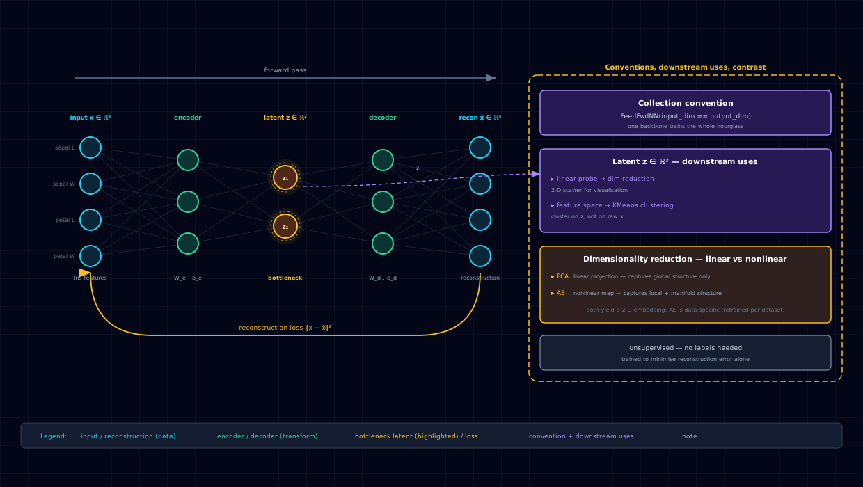
Both autoencoders are constructed via the same FeedFwdNN(input_dim=4, output_dim=4,
hidden_dims=[\ldots]) trick. The middle of hidden_dims is the bottleneck — the only learned
representation.
| Candidate | Topology | Encoder / Decoder | Role |
|---|---|---|---|
| PCA | linear, closed-form | n/a | The variance-maximizing baseline |
AE shallow [2] |
4 → 2 → 4 |
4 → 2 / 2 → 4 |
Tests whether any non-linearity helps |
AE deeper [3, 2, 3] |
4 → 3 → 2 → 3 → 4 |
4 → 3 → 2 / 2 → 3 → 4 |
Tests whether depth helps further |
The shared contract — everything held constant across the two AE candidates:
- Net:
Nets.FEED_FWDwithinput_dim == output_dim == 4 - Loss field:
Losses.CROSS_ENTROPY(cosmetic — unused; theautoencoder_stepcomputes its own MSE) - Optimizer:
Optims.ADAM,max_lr=5e-3,weight_decay=0.0,momentum=(0.9, 0.999) - Device:
Devices.CPU - Epochs:
300(full run) or5(SMOKE_TEST=1for CI; AE under-trains visibly) - Batch size:
16 - Dropout:
0.0 - Activation:
Activations.RELU - Seed:
0(re-pinned before each candidate) train_step_fn:autoencoder_step— MSE reconstruction, ignoresY
The data plumbing: 70/15/15 stratified split (train=104, val=23, test=23), MinMax-scaled to
[0, 1] so reconstruction MSE is on a bounded scale. The val loader exists because
NNTrainParams expects one, but the val loss is also computed via the custom step — the same
reconstruction MSE, just on the val batch.
The a priori expectation: PCA should be hard to beat on iris because the species variance is essentially aligned with petal-length and petal-width (the top-2 PCs). The shallow AE should match PCA roughly. The deeper AE's extra capacity should overfit on 150 samples and may lose species separation in the bottleneck. The results section either confirms or refutes this.
8.20.5 Code walkthrough¶
8.20.5.1 Autoencoder construction¶
def make_autoencoder(hidden_dims):
    return NNModel(
        net_params=NNParams(
            input_dim=X.shape[1],
            output_dim=X.shape[1],
            hidden_dims=hidden_dims,
            dropout_prob=0.0,
            activation=Activations.RELU,
        ),
        # loss is unused — autoencoder_step computes its own MSE loss
        params=NNModelParams(
            net=Nets.FEED_FWD,
            device=DEVICE,
            loss=Losses.CROSS_ENTROPY,
        ),
    )
The loss=Losses.CROSS_ENTROPY is cosmetic — it is never invoked because the custom step
computes its own MSE. NNModelParams requires the field to be present, so the notebook sets it
to a placeholder. This is a known rough edge of the nnx API for unsupervised training.
8.20.5.2 The train_step_fn contract¶
def autoencoder_step(ctx):
    """MSE reconstruction loss; ignore y. Adapted from
    nnx/examples/05_custom_train_step_autoencoder.py."""
    m = ctx.model
    m.net.train()
    m.net.zero_grad()
    X_in, _ = m.net.unpack_batch(ctx.batch)
    X_in = tuple(x.to(m.device) for x in X_in)
    recon = m.net(*X_in)
    loss = F.mse_loss(recon, X_in[0])
    loss.backward()
    ctx.optimizer.step()
    loss_val = float(loss.detach())
    return NNEvaluationDataPoint(
        loss=loss_val, error=loss_val,
        accuracy=0.0, f1=0.0, recall=0.0, precision=0.0,
    )
The ctx argument (a TrainStepContext) exposes model, optimizer, batch, batch_idx,
accumulate_grad_batches, grad_clip_norm. The function does the full forward → loss →
backward → step dance manually and returns an NNEvaluationDataPoint so the framework's
loss/error tracking stays uniform. The error=loss_val line is intentional — for unsupervised
reconstruction, loss is the error. The accuracy/f1/recall/precision=0.0 fields are
placeholders that satisfy the EDP contract; they're never consumed.
The m.net.unpack_batch(ctx.batch) call is the canonical way to peel apart the batch inside a
custom step — it handles device movement and dtype normalization consistently with what the
default supervised step does. The trailing _ discards the dummy Y from the loader (which
exists only to satisfy the (X, y) batch contract).
8.20.5.3 Training¶
def train_ae(model):
    return model.train(
        params=NNTrainParams(
            n_epochs=N_EPOCHS,
            train_loader=train_loader,
            val_loader=val_loader,
            optim=NNOptimParams(
                name=Optims.ADAM, max_lr=LR,
                momentum=(0.9, 0.999), weight_decay=0.0,
            ),
        ),
        train_step_fn=autoencoder_step,
    )
train_step_fn=autoencoder_step is the only structural difference from the supervised recipe.
The framework still owns the epoch loop, the val cadence, the iteration-data-point logging, and
the checkpoint schedule — autoencoder_step only owns one forward + backward.
8.20.5.4 Encoder extraction¶
def encode(model, X_np):
    """Run the encoder half of an FFN-autoencoder; return the (N, latent_dim) latent."""
    net = model.net
    net.eval()
    # Find the Linear whose out_features == LATENT_DIM (the bottleneck).
    bottleneck_idx = next(i for i, L in enumerate(net.layers) if L.out_features == LATENT_DIM)
    with torch.no_grad():
        x = torch.from_numpy(X_np).float()
        # Walk the encoder half manually with the model's activation between Linears.
        for i, L in enumerate(net.layers[: bottleneck_idx + 1]):
            x = L(x)
            if i < bottleneck_idx:
                x = F.relu(x)
        return x.numpy()
This is the trick that makes the FeedFwdNN-as-autoencoder pattern work. net.layers is a
ModuleList of Linear layers; the bottleneck is identified by out_features == LATENT_DIM.
The encoder is the prefix of net.layers up to and including the bottleneck, with F.relu
applied between Linears (mirroring what FeedFwdNN.forward does internally). The bottleneck
activation itself is linear — that's the latent.
8.20.5.5 Linear probe¶
def linear_probe(train_z, train_y, test_z, test_y):
    clf = LogisticRegression(max_iter=1000).fit(train_z, train_y)
    return accuracy_score(test_y, clf.predict(test_z))
The probe is LogisticRegression fit on the 2-D train latents and evaluated on the 2-D test
latents. This isolates "how separable are the species in this latent space" from "how good is
the classifier" — a linear probe failing means the latent doesn't linearly separate the
species, regardless of what a fancier classifier might do.
8.20.6 Results¶
On the seeded (random_state=0) 70/15/15 stratified split (train=104, val=23, test=23), with
PCA explained variance [0.833, 0.129] on the train split, the three latents land as:
| Recipe | Latent dim | Test linear-probe accuracy |
|---|---|---|
| PCA | 2 | 82.61% |
AE shallow [2] |
2 | 100.00% |
AE deeper [3, 2, 3] |
2 | 34.78% |
Three observations:
- Shallow AE beats PCA, confirming the non-linearity hypothesis. 100 % linear-probe accuracy on the 23-sample held-out test split means the shallow AE's 2-D latent perfectly linearly separates the three species. The ReLU kink in the encoder adds just enough non-linearity to push the versicolor/virginica boundary into a cleaner configuration than the linear PCA projection.
- Deeper AE collapses, confirming the overfit hypothesis. 34.78 % linear-probe accuracy
on the deeper AE is barely above the majority-class baseline (33 %). The extra capacity in
[3, 2, 3]overfits the reconstruction objective on 104 train samples — the encoder learns a 2-D representation that minimizes reconstruction MSE but does not preserve species-relevant structure. The reconstruction loss is lower than the shallow AE's, but the latent is worse for downstream classification. - PCA's 82.61% is a strong baseline. Iris's variance is essentially aligned with petal dimensions, which separate setosa cleanly from the other two species. The remaining ~17 % gap to perfect is the versicolor/virginica overlap that PCA's linear projection cannot resolve but the shallow AE's non-linear one can.
The latent-space scatter plots (cell 25) make the same point visually: the shallow AE's 2-D plane shows three cleanly separated species clouds, the PCA plane shows setosa cleanly separated but versicolor/virginica overlapping, and the deeper AE's plane shows the three species clouds smeared together. The deeper-AE failure is the pedagogically interesting result — capacity is not free, and a reconstruction objective does not automatically preserve the structure downstream tasks care about.
8.20.7 Pitfalls & edge cases¶
- Deeper AE can lose to shallow. At iris scale (150 samples), the extra capacity in
[3, 2, 3]often overfits the reconstruction objective and loses species-separation in the bottleneck. The §6.3 prose owns this. The shallow[2]is the safer default for small datasets. - Linear-probe accuracy swings run-to-run. With only 22-23 test samples, single-class mis-predictions move the accuracy by ~4.5 percentage points. The qualitative ordering (shallow AE > PCA on this seed) is stable; the absolute numbers aren't. Read the 100 % and 34.78 % as "on this split," not as "on iris."
- No explicit encoder/decoder modules. Latents are extracted by walking
net.layers[: bottleneck_idx + 1]manually withF.relubetween Linears. This mirrors whatFeedFwdNN.forwarddoes internally; if you change the activation inNNParams, also update the latent-extractor in §5.3 or the latent will be inconsistent with what the network actually computes during training. - MSE on MinMax-scaled
[0, 1]inputs. Switching toStandardScaler(mean 0, std 1) would change the absolute reconstruction-loss scale but not the species-separation ranking. MinMax is chosen here so reconstruction MSE is bounded and comparable across the two AE variants. - The
lossfield inNNModelParamsis cosmetic whentrain_step_fnis used. The custom step computes its own MSE; the framework never invokes the configuredLosses.CROSS_ENTROPY. This is a known rough edge — downstream unsupervised notebooks should follow the same pattern and not be confused by the placeholder value. - Stratify the split. At 150 samples times 15 % test, a default random split can plausibly
miss a whole class. The
stratify=argument ontrain_test_splitis load-bearing. - The AE is not a checkpoint producer.
runs/is gitignored, so a fresh CI checkout can't load this notebook's AE checkpoint. The siblingclustering-iris-kmeans-vs-ae-pytorchnotebook retrains the AE inline for exactly this reason — no cross-notebook checkpoint dependency at runtime.
8.20.8 Extensions¶
- Add a denoising autoencoder variant. Inject Gaussian noise into the encoder input and require reconstruction of the clean input; tests whether the AE learns more robust representations than the deterministic reconstruction objective alone.
- Swap the bottleneck for a 3-D latent and visualize in 3-D. Tests whether the species-separation ranking (shallow > PCA > deeper) holds at higher latent dim, or whether the deeper AE's overfit trap disappears with more bottleneck capacity.
- Add a variational autoencoder (VAE) variant. The KL-divergence regularizer on the bottleneck would directly penalize the kind of overfit-to-reconstruction failure mode the deeper AE exhibits; the comparison would test whether VAE-style regularization preserves species-separation in the bottleneck.
- Persist and reload the AE via
NNCheckpoint.load(run=..., type=Checkpoints.BEST). The notebook uses the liverunobject because the AE trains in seconds; a follow-up that saves the AE to./runs/and reloads its best checkpoint would exercise the serialization contract that the longer-running generative tasks depend on. (Caveat:runs/is gitignored, so this is a local-only follow-up unless the checkpoint is published out-of-band.) - Scale the recipe to a higher-dimensional dataset. Iris's 4 → 2 projection is too easy for the depth-vs-shallowness trade-off to generalize; the same pattern on a 30-D or 100-D dataset would show the deeper AE paying off where PCA leaves substantial structure on the table.