8.2 Tabular regression — Diabetes MLP

A comprehensive walk-through of notebooks/tabular_regression-diabetes-mlp-pytorch/ — the first regression task in ml-eng-lab. The collection's other tabular, image, and node tasks are all classification; regression is structurally different in three places (one-output head, MSE loss, R²/MAE/RMSE metrics), and this notebook lands the slot and walks through each difference explicitly so the recipe is reusable for the future regression tasks on the roadmap (anomaly-detection autoencoders, time-series forecasting).

The notebook is Tier-A — CPU re-runs in ~22 seconds and it is re-executed end-to-end in CI on every pull request. It is also the first notebook that cannot use nnx.NNTabularDataset, because that helper hard-coerces targets to torch.long and is therefore classification-only. §3.3 of the notebook builds the DataLoaders by hand with dtype=torch.float32 targets shaped (N, 1); the present page explains why that workaround remains necessary under the retained NNx 0.2.0 contract. Issue #61 validated 0.2.2's optional target_dtype=torch.float32 surface but did not adopt it because the recommended Atlas runtime remains on 0.2.0.

The falsifiable hypothesis tested by the notebook is that on a 442-sample classical-statistics benchmark, linear and KNN baselines are surprisingly hard to beat — the MLPs are interesting not because they win, but because they offer a uniform nnx.NNModel recipe that scales to the much-bigger-than-diabetes data settings where the baselines run out of capacity.

8.2.1 Problem & motivation

The diabetes dataset (sklearn.datasets.load_diabetes) is 442 patients × 10 numeric features (age, sex, BMI, blood pressure, six blood serum measurements — all already mean-centered and unit-variance-normalized in the sklearn version) with a continuous target = disease-progression score one year after baseline. The target ranges over [25.0, 346.0] with mean \(152.1\) and standard deviation \(77.0\) on the recorded run, so the "predict within ±one standard deviation" floor is already a substantial spread.

This notebook exists for three reasons:

1. Land the first regression slot. Classification and regression diverge at the output head, the loss, and the metrics; the notebook makes each divergence first-class. nnx exposes the right primitives (output_dim=1, Losses.MEAN_SQUARED_ERROR, manual DataLoaders), and the notebook is the canonical demo of composing them.
2. Surface a real footgun in the nnx API. nnx.NNTabularDataset coerces targets to torch.long — it is hard-coded for classification. Using it for regression silently truncates the fractional disease-progression scores and then crashes inside the loss computation when the network outputs floats. The notebook's §3.3 builds the loaders manually and the README §6 records the gotcha for downstream regression notebooks.
3. Head-to-head against classical baselines. sklearn.LinearRegression (closed-form OLS) and sklearn.KNeighborsRegressor(k=5) (smoothed local average) bracket the MLP story from both ends — the closed-form floor and the classical non-linear floor. The MLPs are then evaluated against both, not just against each other.

The falsifiable hypothesis is that diabetes is small enough that linear regression is well-conditioned and the MLPs cannot extract additional non-linear signal before overfitting the 308-sample train split. The results section either confirms or refutes this.

8.2.2 Concepts

Concept	Where it shows up
Regression	Continuous disease-progression target; one output unit, not n_classes logits
MSE loss	Losses.MEAN_SQUARED_ERROR — the recipe-defining choice for the loss head
R² / RMSE / MAE	sklearn.metrics.{r2_score, mean_squared_error, mean_absolute_error}
StandardScaler	Re-fit on train only; applied to val + test (anti-leakage)
MLP (multi-layer perceptron)	nnx.FeedFwdNN with hidden_dims swept over [8] and [32, 16]
Manual DataLoader construction	TensorDataset + DataLoader because NNTabularDataset is classification-only
Closed-form OLS baseline	sklearn.LinearRegression — the linear floor to beat
Local-averaging baseline	sklearn.KNeighborsRegressor(k=5) — the classical non-linear floor
Reproducibility	nnx.set_seed(0) pins Python random, NumPy, PyTorch CPU + CUDA + cuDNN

The nnx flat re-exports consumed are: NNModel, NNParams, NNModelParams, NNTrainParams, NNOptimParams, Devices, Losses, Nets, Optims, Activations, set_seed. The enums (Nets.FEED_FWD, Losses.MEAN_SQUARED_ERROR, Optims.ADAM, Devices.CPU, Activations.RELU) make the model + training contract read as configuration rather than magic strings. Notice that NNTabularDataset is not in this list — the regression case has to drop one layer of abstraction.

8.2.3 Mathematical formulation

The regressor produces a scalar output \(\hat{y} = f_\theta(x) \in \mathbb{R}\) — the predicted disease-progression score for the input feature vector \(x\). The training objective is the mean-squared error between prediction and ground-truth target:

\[ \mathcal{L}(\theta) = \frac{1}{N} \sum_{i=1}^{N} \bigl(y_i - \hat{y}_i\bigr)^2. \]

nnx selects this loss via Losses.MEAN_SQUARED_ERROR; the framework pairs it with the single-output head of FeedFwdNN(output_dim=1), so the notebook never instantiates either by hand. The targets must be shaped (N, 1) to match the network output — (N,) would broadcast inside the loss and silently produce a different reduction.

The optimizer is Adam with learning rate \(\eta = 10^{-2}\), weight decay \(10^{-4}\), and momentum moments \((\beta_1, \beta_2) = (0.9, 0.999)\):

\[ m_t = \beta_1 m_{t-1} + (1-\beta_1) g_t, \quad v_t = \beta_2 v_{t-1} + (1-\beta_2) g_t^2, \quad \theta_t \leftarrow \theta_{t-1} - \eta \frac{\hat{m}_t}{\sqrt{\hat{v}_t} + \epsilon}. \]

Evaluation uses three complementary metrics. The coefficient of determination \(R^2\) is the fraction of variance explained, relative to the constant-\(\bar{y}\) predictor:

\[ R^2 = 1 - \frac{\sum_i (y_i - \hat{y}_i)^2}{\sum_i (y_i - \bar{y})^2}. \]

\(R^2 = 1\) is a perfect predictor; \(R^2 = 0\) is "no better than predicting the mean"; \(R^2 < 0\) is "worse than the mean" — possible on a held-out test split even for a reasonable model. Root mean-squared error \(\mathrm{RMSE} = \sqrt{\mathcal{L}}\) returns the error to the target units (here, progression-score points), and mean absolute error \(\mathrm{MAE} = \frac{1}{N}\sum_i |y_i - \hat{y}_i|\) is the robust-to-outliers sibling.

8.2.4 Architecture

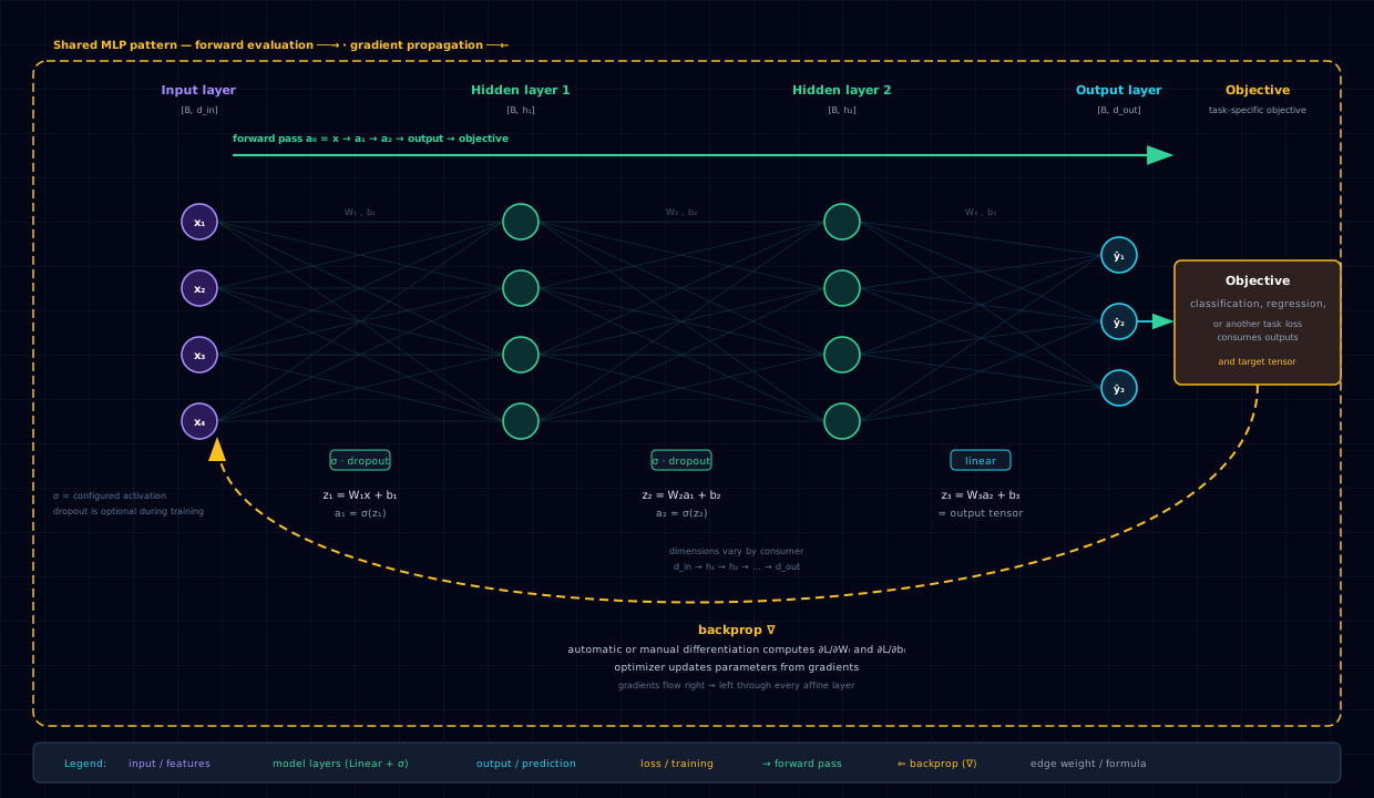
The network family is Nets.FEED_FWD (nnx.FeedFwdNN): an input layer of ten units (one per feature), zero or more hidden layers with ReLU activation, and a one-unit output layer consumed directly by MSE — there is no softmax and no activation on the output head. The notebook trains two MLP topologies head-to-head against two classical baselines, holding everything else fixed:

Candidate	Topology	Parameters (rough)	Role
LinearRegression	closed-form OLS	\(11\) (10 weights + bias)	The linear floor to beat
KNN (\(k=5\))	lazy local average	\(0\) (stores train)	The classical non-linear floor
MLP small [8]	\(10 \cdot 8 + 8 \cdot 1 = 88\)	89	Tests whether any non-linearity helps
MLP deep [32, 16]	\(10 \cdot 32 + 32 \cdot 16 + 16 \cdot 1 = 624\)	625	Tests whether depth helps further

The shared contract — everything held constant across the two MLP candidates:

• Net: Nets.FEED_FWD
• Loss: Losses.MEAN_SQUARED_ERROR
• Optimizer: Optims.ADAM, max_lr=1e-2, weight_decay=1e-4, momentum=(0.9, 0.999)
• Device: Devices.CPU
• Epochs: 200 (full run) or 5 (SMOKE_TEST=1 for CI)
• Batch size: 32
• Dropout: 0.0 — tiny model plus tiny dataset means dropout would starve them
• Activation: Activations.RELU
• Seed: 0 (re-pinned inside train_mlp before each candidate)

The data plumbing is identical across candidates: three manual DataLoaders (one per split), each wrapping a TensorDataset of (float32 features, float32 target unsqueezed to (N, 1)). The train loader shuffles; the val and test loaders don't. The StandardScaler is fit on the train split only and applied to val and test.

The a priori expectation, recorded before training: LinearRegression is hard to beat on 442 samples; KNN trails slightly because \(k=5\) averages over a wide neighborhood in the sparse 10-D feature space; the small MLP can match or slightly beat KNN; the deep MLP is usually worse because it overfits the 308-sample train split before it extracts any non-linear signal. The results section either confirms or refutes this.

8.2.5 Code walkthrough

8.2.5.1 Data loading

diabetes = load_diabetes()
X, y = diabetes.data.astype('float32'), diabetes.target.astype('float32')

Features are already mean-centered and unit-variance-normalized in the sklearn version (per-feature std ≈ \(1/\sqrt{442} \approx 0.048\)). The cast to float32 matters — MSE between float64 features and a float32 network output silently promotes and wastes memory.

8.2.5.2 Splits and scaling

X_trainval, X_test, y_trainval, y_test = train_test_split(X, y, test_size=0.15, random_state=0)
X_train, X_val, y_train, y_val = train_test_split(X_trainval, y_trainval, test_size=15/85, random_state=0)

scaler = StandardScaler()
X_train_s = scaler.fit_transform(X_train).astype('float32')
X_val_s   = scaler.transform(X_val).astype('float32')
X_test_s  = scaler.transform(X_test).astype('float32')

The split is 70/15/15: train=308, val=67, test=67. StandardScaler is fit on the train split only and then applied to val and test — the canonical anti-leakage pattern. Note that the split here is not stratified: regression targets are continuous, so stratification is inapplicable. The random_state=0 pin is what makes the recorded numbers reproducible.

8.2.5.3 Manual DataLoader construction (the regression workaround)

def make_loader(X, y, batch_size, shuffle):
    # MSE loss expects a target tensor of shape (N, 1) matching the
    # network output_dim=1 (not a class index).
    return DataLoader(
        TensorDataset(
            torch.from_numpy(X).float(),
            torch.from_numpy(y).float().unsqueeze(-1),
        ),
        batch_size=batch_size,
        shuffle=shuffle,
    )

This is the load-bearing regression workaround. nnx.NNTabularDataset would coerce the target to torch.long, silently truncating the fractional disease-progression scores and then crashing inside MSE. The unsqueeze(-1) is the second non-obvious bit: MSE between a network output of shape (B, 1) and a target of shape (B,) would broadcast and produce a different reduction than intended. The notebook's docstring even records the workaround: "For regression, prefer to construct the DataLoaders yourself and pass them through NNTrainParams."

8.2.5.4 MLP construction

def make_mlp(hidden_dims):
    return NNModel(
        net_params=NNParams(
            input_dim=X.shape[1],
            output_dim=1,                       # continuous scalar
            hidden_dims=hidden_dims,
            dropout_prob=0.0,
            activation=Activations.RELU,
        ),
        params=NNModelParams(
            net=Nets.FEED_FWD,
            device=DEVICE,
            loss=Losses.MEAN_SQUARED_ERROR,      # the recipe-defining choice
        ),
    )

output_dim=1 and loss=Losses.MEAN_SQUARED_ERROR are the two differences from the classification recipe. Everything else — input_dim, hidden_dims, dropout_prob, activation, the Nets.FEED_FWD selection — is identical to the Iris classification notebook.

8.2.5.5 Training loop

def train_mlp(hidden_dims):
    nnx.set_seed(0)
    m = make_mlp(hidden_dims)
    r = m.train(
        params=NNTrainParams(
            n_epochs=N_EPOCHS,
            train_loader=train_loader,
            val_loader=val_loader,
            optim=NNOptimParams(
                name=Optims.ADAM, max_lr=LR,
                momentum=(0.9, 0.999), weight_decay=1e-4,
            ),
        ),
    )
    return m, r

mlp_small, run_small = train_mlp(SMALL_HIDDEN)
mlp_deep,  run_deep  = train_mlp(DEEP_HIDDEN)

The seed is re-pinned inside train_mlp so identical seeds produce identical weight inits — the only difference between candidates is hidden_dims. The NNTrainParams now takes train_loader and val_loader directly as constructor arguments (the classification recipe uses a fluent .with_train_loader(...) pattern; both are valid).

8.2.5.6 Evaluation

preds_lr  = linreg.predict(X_test_s)
preds_knn = knn.predict(X_test_s)
preds_sm  = mlp_small.predict(X_test_s).logits.squeeze(-1)
preds_dp  = mlp_deep.predict(X_test_s).logits.squeeze(-1)

The two MLP .predict(...) calls return a prediction object whose .logits field carries the raw network output — the squeeze(-1) collapses the (N, 1) trailing dim back to (N,) so the metric functions see 1-D arrays as they expect. The two sklearn baselines return (N,) directly.

def metrics(y_true, y_pred):
    return {
        'MSE':  mean_squared_error(y_true, y_pred),
        'RMSE': float(np.sqrt(mean_squared_error(y_true, y_pred))),
        'MAE':  mean_absolute_error(y_true, y_pred),
        'R2':   r2_score(y_true, y_pred),
    }

The four metrics bracket different failure modes: \(R^2 < 0\) flags "worse than the mean"; \(\mathrm{MAE} \ll \mathrm{RMSE}\) flags heavy-tailed residuals (RMSE is dominated by the largest error); comparing MSE across candidates in the original target units is what makes the headline comparable to the dataset's \(77.0\) target standard deviation.

8.2.6 Results

On the seeded (random_state=0) 70/15/15 split (train=308, val=67, test=67), the four candidates land as:

Candidate	MSE	RMSE	MAE	R²
LinearRegression (sklearn)	3703.4	60.86	47.56	0.225
KNeighborsRegressor (k=5)	4645.0	68.15	53.53	0.028
nnx MLP small [8]	4019.5	63.40	48.43	0.159
nnx MLP deep [32, 16]	4158.4	64.49	48.96	0.130

Three observations:

1. LinearRegression wins, confirming the small-data hypothesis. \(R^2 = 0.225\) on the 67-sample held-out test split is the headline. The diabetes target carries substantial irreducible measurement noise (1-year disease progression is noisy biologically), so even closed-form OLS leaves more than 75 % of the variance unexplained — this is a property of the dataset, not of the model.
2. KNN trails by a wide margin. \(R^2 = 0.028\) is barely above the constant-mean predictor. With 10 features and 308 train samples, \(k=5\) averages over a neighborhood that spans a substantial fraction of the input space — the local-average assumption breaks down in this relatively-high-dimensional, relatively-low-sample regime (the curse of dimensionality at work).
3. The MLPs rank between the two baselines, and small beats deep. MLP small [8] at \(R^2 = 0.159\) is better than KNN but worse than linear; MLP deep [32, 16] at \(R^2 = 0.130\) is worse than the small one. The deeper network has 7× the parameters of the small one and overfits the 308-sample train split before it can extract any non-linear signal that generalizes.

The predicted-vs-actual scatter (cell 24) makes the same point visually: the LinearRegression points cluster most tightly around the y = x diagonal, the KNN points spread widely, and the two MLP residuals show structure (the predicted-vs-actual cloud has curvature) that suggests the MLPs are picking up noise as if it were signal. The residual scatter confirms mean-zero-ish residuals in all four cases, so none of the models is systematically biased — the differences are pure variance.

8.2.7 Pitfalls & edge cases

• nnx.NNTabularDataset is classification-only. Its __post_init__ coerces targets to torch.long; using it for regression silently truncates fractional targets and then crashes inside MSE. The notebook's §3.3 builds the loaders manually with dtype=torch.float32 targets, and downstream regression notebooks (anomaly-detection autoencoder, time-series forecasting) will need the same workaround until the upstream nnx API gains a regression mode.
• Targets must be shaped (N, 1) to match output_dim=1. Passing (N,) targets into MSE against a (B, 1) network output broadcasts across the trailing dim and silently produces a different reduction than intended. The unsqueeze(-1) in make_loader is load-bearing.
• Do not stratify the split. Stratification is a classification concept — regression targets are continuous, so stratify= is inapplicable. Pin random_state=0 for reproducibility instead.
• EarlyStopping's default monitor is the wrong one for regression. The default monitor is val_edp.error — for classification (lower error = better, mode="min"). For regression the optional error field on the evaluation data point is unset (None); the right monitor is val_edp.loss. The notebook does not use EarlyStopping (to keep the budget predictable), but downstream regression notebooks should pass monitor="val_edp.loss" explicitly if they do.
• Fit the scaler on train only. Applying fit_transform to val or test leaks their feature ranges into training and inflates the headline metric. The notebook is careful to call scaler.fit_transform(X_train) and then scaler.transform(...) on val and test. The sklearn version of diabetes is already centered and scaled, but the re-scaling step makes the code path generalize to non-pre-scaled data.
• More MLP capacity is not always better. hidden_dims=[32, 16] (625 params) underperforms hidden_dims=[8] (89 params) on this 308-sample train split. The deep MLP overfits before it extracts any non-linear signal that generalizes. At 442 samples, diabetes is a classical-statistics benchmark, not a deep-learning playground.
• Read \(R^2\) on a single hold-out split with skepticism. The 67-sample test split means each prediction contributes roughly \(1.5\%\) of the variance. A different seed would move the headline by a percentage point or two in either direction.

8.2.8 Extensions

• Add k-fold cross-validation. Replaces the single-split \(R^2\) with a mean-plus-spread over five folds; closes the "on this split" caveat in the pitfalls section at the cost of five times the training compute (still seconds on CPU for diabetes).
• Huber loss instead of MSE. Losses.HUBER (when available in nnx) is robust to the heavy-tailed residuals that dominate diabetes predictions; the comparison would test whether the MLPs' disadvantage against linear regression shrinks under a robust objective.
• Scale the same pattern to a bigger-than-diabetes regression task. The whole point of landing the regression recipe here is to reuse it on a dataset where the MLP capacity actually pays off — e.g., the planned anomaly-detection autoencoder (reconstruction as regression) or time-series forecasting tasks in the roadmap.
• Add EarlyStopping(monitor="val_edp.loss"). Lets the MLPs auto-stop when val loss plateaus, recovering some of the overfit gap. The notebook uses a fixed N_EPOCHS=200 instead for budget predictability in CI; a follow-up that swaps in early stopping would show the validation curve shape directly.
• Feature engineering. Add interaction terms (bmi × bp, s5 × s6) before the MLP; tests whether the linear model's additive-feature assumption is the binding constraint, or whether the irreducible noise floor is.