8.10 Diffusion — DDPM on MNIST¶

A comprehensive walk-through of notebooks/diffusion-mnist-ddpm-pytorch/ — the canonical in-repo exercise of the nnx diffusion stack (NoiseSchedulers.LINEAR, DiffusionMLP, diffusion_train_step_factory, sample). This page is the deep-dive companion to the task notebook: it states the problem, builds the math, dissects the architecture, reads the code top to bottom, reports the measured results, and catalogues the pitfalls and extensions that govern the recipe.

The notebook is Tier-A — CPU re-runs in roughly nineteen seconds and it is re-executed end-to-end in CI on every pull request. It is intentionally tiny: a three-layer MLP denoiser on flattened 784-D pixels, \(T = 100\) timesteps, three epochs on CPU. At this scale and budget the generated digits are blurry and mode-mixed; the point is the pipeline (schedule → train step → sampler), not generation quality. The same three calls with a U-Net denoiser in place of DiffusionMLP produces a much better generator with no other plumbing changes.

8.10.1 Problem & motivation¶

DDPM (Ho et al., 2020) is the foundational diffusion-model recipe: train a denoiser network \(\varepsilon_\theta\) to predict the noise added to a clean image at a randomly-sampled noise level \(t \in [0, T)\). Generation is the reverse process — start from pure Gaussian noise, run the denoiser iteratively backward from \(t = T-1\) down to \(t = 0\), and the result is a sample from the learned distribution. The training objective is a simple mean-squared error on the noise vector; the generative power comes entirely from the schedule + the iterative reverse process.

The nnx megamerge ships the full stack as four composable primitives:

NoiseSchedulers.LINEAR(T=...) — builds a NoiseSchedule with the standard linear \(\beta\)-schedule.
DiffusionMLP(input_dim, hidden_dims, time_embed_dim) — the denoiser. Takes \((x_t, t)\), returns predicted \(\varepsilon\). A sinusoidal time embedding is fused with the noisy image internally.
diffusion_train_step_factory(schedule) — produces the train_step_fn implementing the noise-prediction objective \(\text{MSE}(\varepsilon_\theta(x_t, t), \varepsilon)\).
sample(model, schedule, shape, ...) — runs the reverse-diffusion loop.

This notebook exists for two reasons:

End-to-end exercise of the megamerge diffusion stack. It is the in-repo smoke test that all four primitives work together on the simplest possible denoiser architecture.
Architecture-agnostic plumbing. The MLP denoiser keeps the diffusion plumbing visible — no U-Net convolutions or skip connections obscure the schedule/step/sampler contract. The §6.3 scaling levers are exactly "swap the denoiser, keep the rest."

The falsifiable hypothesis tested by the notebook is that, at this deliberately tiny budget, the noise-prediction loss decreases monotonically (the denoiser is learning to invert the forward noising process) while the generated samples remain low-fidelity and mode-mixed — isolating capacity as the bottleneck rather than the pipeline.

8.10.2 Concepts¶

Concept	Where it shows up
Forward noising process	`NoiseSchedule` closes-form samples \(x_t\) given \(x_0\), \(t\), and \(\varepsilon\)
Linear \(\beta\)-schedule	`NoiseSchedulers.LINEAR(T=100)`
Noise-prediction objective	`diffusion_train_step_factory(schedule)` — predict \(\varepsilon\), not \(x_0\)
Sinusoidal time embedding	`time_embed_dim=32` fused into the MLP denoiser
Reverse-diffusion sampling	`sample(model, schedule, shape=(16, 784))`
EMA / ancestral sampling	DDPM ancestral update with learned \(\varepsilon_\theta\)
`.net` substitution	`NNModel` shell with placeholder `FeedFwdNN`, then `model.net = DiffusionMLP(...)`
Reproducibility	`nnx.set_seed(0)`

The nnx surface consumed is DiffusionMLP, NoiseSchedulers, diffusion_train_step_factory, sample, NNModel, NNDataset, NNModelParams, NNParams, NNTrainParams, NNOptimParams, Activations, Devices, Losses, Nets, Optims, and set_seed. The NNModelParams carries a Losses.CROSS_ENTROPY placeholder that the diffusion step ignores — it computes its own MSE.

8.10.3 Mathematical formulation¶

The forward (noising) process is a fixed Markov chain that progressively corrupts a clean image \(x_0\) toward isotropic Gaussian noise:

\[ q(x_t \mid x_0) = \mathcal{N}\!\left(x_t;\, \sqrt{\bar{\alpha}_t}\, x_0,\, (1 - \bar{\alpha}_t)\, I\right), \]

with the closed-form reparameterization used for training:

\[ x_t = \sqrt{\bar{\alpha}_t}\, x_0 + \sqrt{1 - \bar{\alpha}_t}\, \varepsilon, \qquad \varepsilon \sim \mathcal{N}(0, I). \]

The linear schedule defines \(\beta_t\) interpolating linearly between two endpoints, \(\alpha_t = 1 - \beta_t\), and \(\bar{\alpha}_t = \prod_{s=1}^{t} \alpha_s\). With \(T = 100\) the cumulative product \(\bar{\alpha}_T\) is small enough that \(x_T\) is effectively pure noise.

The training objective is the simplified noise-prediction loss of Ho et al.:

\[ \mathcal{L}(\theta) = \mathbb{E}_{t \sim \mathcal{U}\{0, T-1\},\, x_0,\, \varepsilon} \;\Big\lVert \varepsilon - \varepsilon_\theta(x_t, t) \Big\rVert_2^{\,2}. \]

The timestep \(t\) is sampled uniformly per image per step (one \(t\) per image in the batch), the noisy sample \(x_t\) is constructed by the closed-form forward, and the denoiser \(\varepsilon_\theta\) predicts the noise. No labels are used — this is unconditional generation.

The denoiser fuses image and timestep via a sinusoidal time embedding. With time_embed_dim=32, the scalar \(t\) is mapped to a 32-D vector by a fixed sinusoidal positional encoding, projected, and concatenated (or added) into the MLP alongside the noisy input. This is how the denoiser knows which noise level it is denoising.

Generation is the ancestral reverse process. Starting from \(x_T \sim \mathcal{N}(0, I)\) and iterating \(t = T-1, \ldots, 0\):

\[ x_{t-1} = \frac{1}{\sqrt{\alpha_t}} \left( x_t - \frac{\beta_t}{\sqrt{1 - \bar{\alpha}_t}}\, \varepsilon_\theta(x_t, t) \right) + \sigma_t z, \qquad z \sim \mathcal{N}(0, I), \]

with \(\sigma_t\) the schedule-defined reverse noise scale; the sample(...) primitive runs this loop. After \(T\) steps the output is a sample from the learned distribution.

8.10.4 Architecture¶

DDPM diffusion

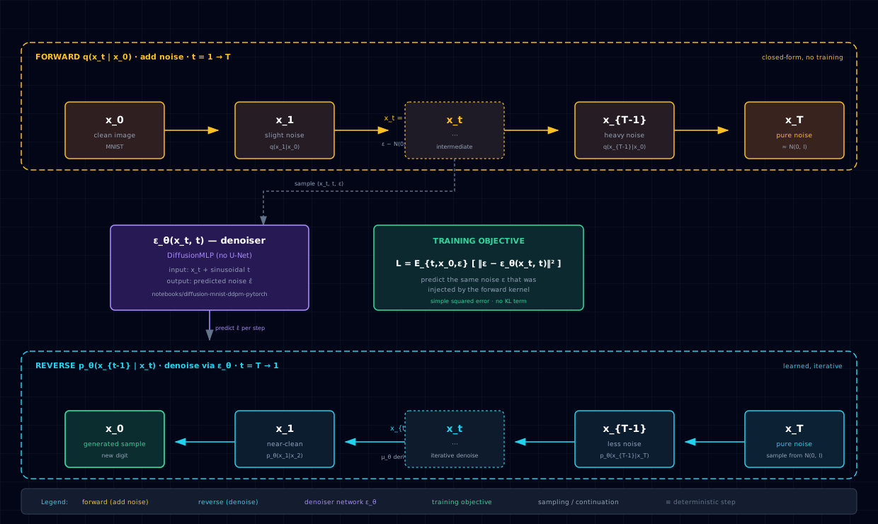
DiffusionMLP(input_dim=784, hidden_dims=[256, 256], time_embed_dim=32) is a three-layer MLP denoiser. The contract is (x_t, t) → ε̂:

Stage	Shape	Role
Input	784	Flattened 28×28 noisy image \(x_t\)
Time embedding	scalar → 32	Sinusoidal positional encoding of \(t\), projected
Hidden	784 → 256 → 256	MLP on the (image ⊕ time-embedding) fused input
Output	256 → 784	Predicted noise \(\hat{\varepsilon}\), same shape as input
Parameters	—	477,488

The denoiser is built inside the NNModel shell: a placeholder FeedFwdNN is constructed purely so .train() scaffolding (optimizer, scheduler, callbacks, NNRun) is available, then model.net = DiffusionMLP(...).to(model.device) swaps it out. The placeholder's Losses.CROSS_ENTROPY is unused — the diffusion step computes its own MSE.

The shared training contract:

Net: Nets.FEED_FWD shell, then model.net = DiffusionMLP(...).
Schedule: NoiseSchedulers.LINEAR(T=100).
Train step: diffusion_train_step_factory(schedule) (noise-prediction MSE).
Optimizer: Optims.ADAM, max_lr=2e-3, momentum=(0.9, 0.999), weight_decay=0.0.
Device: Devices.CPU.
Epochs: 3 (full run) or 1 (SMOKE_TEST=1 for CI).
Batch size: 128 (the train loader is rebuilt at this granularity — see pitfalls).
Seed: 0.

The a priori expectation: at three epochs the noise-prediction loss should fall noticeably (the denoiser learns to invert the forward noising), but sampled digits will remain blurry and mode-mixed because the MLP denoiser on flattened pixels cannot exploit the spatial structure that a U-Net would. The pipeline working is the headline; the generation quality is the capacity bottleneck.

8.10.5 Code walkthrough¶

8.10.5.1 Denoiser construction and `.net` substitution¶

model = NNModel(
    net_params=NNParams(input_dim=IMG_DIM, output_dim=IMG_DIM,
                        hidden_dims=[32], dropout_prob=0.0,
                        activation=Activations.RELU),
    params=NNModelParams(net=Nets.FEED_FWD, device=DEVICE,
                         loss=Losses.CROSS_ENTROPY),   # unused by the diffusion step
)
model.net = DiffusionMLP(input_dim=IMG_DIM, hidden_dims=DENOISER_HIDDEN,
                         time_embed_dim=TIME_EMBED_DIM).to(model.device)

The placeholder FeedFwdNN is never executed — it exists only to provide the NNModel scaffolding (optimizer wiring, learning-rate scheduler, the NNRun history object). The real denoiser replaces .net. Note input_dim == output_dim == 784 for diffusion: the denoiser predicts a noise vector the same shape as the image.

8.10.5.2 Schedule + custom train step¶

schedule = NoiseSchedulers.LINEAR(T=T)
step_fn = diffusion_train_step_factory(schedule)

run = model.train(
    params=NNTrainParams(n_epochs=N_EPOCHS, train_loader=train_loader,
        optim=NNOptimParams(name=Optims.ADAM, max_lr=LR,
                            momentum=(0.9, 0.999), weight_decay=0.0)),
    train_step_fn=step_fn,
)

The factory wires the schedule into a train_step_fn(ctx) that (1) samples a random \(t \in [0, T)\) per image, (2) computes \(x_t = \sqrt{\bar{\alpha}_t}\, x_0 + \sqrt{1 - \bar{\alpha}_t}\, \varepsilon\), (3) forwards \(\varepsilon_\theta(x_t, t) \to \hat{\varepsilon}\), (4) backprops \(\text{MSE}(\hat{\varepsilon}, \varepsilon)\). The loop is otherwise identical to a supervised classifier's — only the train step differs.

8.10.5.3 Sampling and display un-normalization¶

samples = sample(model, schedule, shape=(N_SAMPLES_GRID, IMG_DIM))
samples_img = samples * DS_STD + DS_MEAN
samples_img = samples_img.clamp(0, 1).view(N_SAMPLES_GRID, 28, 28).numpy()

sample(...) runs the full reverse-diffusion loop and returns a (16, 784) array. The training data was Normalize(mean=0.1307, std=0.3081)-scaled, so the samples live in that normalized space; multiplying back by DS_STD and adding DS_MEAN maps them into roughly \([0, 1]\) before clamping for display. Skipping this step yields visibly-wrong pixel ranges, not a different generative outcome.

8.10.6 Results & analysis¶

On the recorded three-epoch run (seed 0, batch size 128, Adam at lr=2e-3), the metrics land as:

Metric	Value
Denoiser parameters	477,488
Timesteps \(T\)	100
Iterations	1,266 (3 epochs × 422 batches)
Noise-prediction loss	1.0102 → 0.9317
Samples drawn	16 via reverse-diffusion

Three observations:

The denoiser is learning. Noise-prediction loss falls monotonically from 1.0102 to 0.9317 across three epochs. The forward noising process is being inverted — this is the pipeline-level proof of life, independent of generation fidelity.
Samples are blurry and mode-mixed. Individual 28×28 renderings blend digit classes (a "0–7 hybrid" is typical). This is the expected ceiling of an MLP denoiser on flattened pixels at \(T = 100\) with three epochs. The MLP over-fits global pixel statistics rather than the local stroke geometry a U-Net would exploit.
Capacity is the bottleneck, not the pipeline. The schedule, train step, and sampler are architecture-agnostic. Swapping DiffusionMLP for a convolutional U-Net denoiser — with no other changes — produces a much better generator at this same budget.

The pedagogical headline: the nnx megamerge ships a working diffusion stack, and the recipe composes the same way for any denoiser architecture. This notebook is the smoke test on the simplest possible denoiser.

8.10.7 Pitfalls & edge cases¶

NNDataset defaults to whole-split batches. For MNIST that means 54,000 training samples per batch — roughly one iteration per epoch, which gives the denoiser far too few noise-level samples to learn. The notebook passes batch_sizes=(128, None, None) and consumes the wrapper-owned shuffled train loader directly. Same caveat as the MoE and JEPA tasks.
MLP on flattened pixels loses spatial structure. Translation symmetry — the property that lets a U-Net share weights across pixel locations — is invisible to an MLP. Real DDPM generation quality needs a convolutional denoiser; the MLP demo is a pipeline smoke test.
Normalize(mean=0.1307, std=0.3081) shifts the pixel range. Samples are produced in the normalized space and must be un-normalized via samples * DS_STD + DS_MEAN before clamp(0, 1) for display. The diffusion math itself is unchanged either way — this is a display-only fix.
\(T = 100\) is small. Production DDPMs use \(T = 1000\) so the reverse process has more refinement steps. Lower \(T\) trades sample quality for sampling speed; DDIM sampling is the usual mitigation at small \(T\).
Unconditional generation. The diffusion step ignores labels. Class-conditional sampling needs classifier-free guidance or a class-conditional denoiser; the megamerge primitives here are unconditional.
NNModelParams requires a loss field. Even though the diffusion step computes its own MSE, the NNModel shell requires a Losses enum value at construction. The notebook passes Losses.CROSS_ENTROPY as an inert placeholder — it is never used.
Three epochs is far below convergence. Even MLP-scale DDPMs typically need 50+ epochs to produce sharp digits. The Tier-A budget is a smoke test, not a generation-quality claim.

8.10.8 Extensions & references¶

Swap DiffusionMLP for a U-Net denoiser. Keep the schedule, train step, and sampler unchanged; replace only the .net substitution target. This is the single biggest quality lever and the cleanest test that the pipeline is architecture-agnostic.
Raise \(T\) to 1000 and lengthen training. Standard production settings; expect CPU run times in the tens-of-minutes range even at MLP scale.
Switch to DDIM sampling. sample(...) uses ancestral DDPM sampling; DDIM gives comparable quality in far fewer steps — useful when \(T\) is large.
Add class-conditional generation via classifier-free guidance. Requires a class input to the denoiser and a guidance scale at sampling time; turns the unconditional demo into a controllable generator.
References. Ho et al., Denoising Diffusion Probabilistic Models (NeurIPS 2020) — the simplified noise-prediction objective and ancestral sampler used here. Nichol & Dhariwal, Improved Denotting Diffusion Probabilistic Models (ICML 2021) — the learned-variance and cosine-schedule refinements. Song et al., Denoising Diffusion Implicit Models (ICLR 2021) — DDIM. The nnx.DiffusionMLP + diffusion_train_step_factory + sample API is the in-repo surface for this recipe.