8.7 Pruning — MNIST FFN (magnitude sparsity sweep)

A comprehensive walk-through of notebooks/pruning-mnist-ffnn-pytorch/ — the canonical in-repo demo of nnx.prune.magnitude_prune and the magnitude-pruning trade-off curve. This page is the deep-dive companion to the task notebook: it states the problem, builds the pruning math, dissects the bake=True deployable-form contract, reads the code top to bottom, reports the measured accuracy-vs-sparsity sweep, and catalogues the pitfalls and extensions.

The notebook is Tier-A — CPU re-runs in roughly 15 seconds and it is re-executed end-to-end in CI on every pull request. It belongs to the "efficient/compressed MLP" family: where §8.5 edits the architecture and §8.8 changes the bitwidth, pruning keeps the architecture and precision fixed and instead drives the weight tensor sparse, trading a tunable fraction of zeros for accuracy.

8.7.1 Problem & motivation

Weight pruning makes a trained model sparse — most of the weights become exactly zero — so the deployed model is smaller (a sparse tensor compresses to its non-zero entries plus indices) and, on hardware that supports sparse kernels, faster. The simplest recipe is magnitude pruning: in each layer, zero the entries with the smallest absolute value up to a target sparsity \(s\). The small-magnitude weights contribute least to the forward output, the theory goes, so dropping them should cost little accuracy.

The deployment question worth a notebook is the trade-off curve: how aggressive can you go before accuracy collapses? Magnitude pruning's answer is a Pareto frontier — accuracy is flat for a wide range of \(s\), then degrades slowly, then drops off a cliff past the "knee." Finding that knee is the deployment decision.

This notebook exists for two reasons:

1. First in-repo exercise of nnx.prune.magnitude_prune. The nnx release ships magnitude pruning with a bake=True default that writes the zeros into the actual .weight tensor and removes PyTorch's weight_orig + weight_mask reparametrization, so the post-prune state_dict() has the same keys as the unpruned net — the deployable form with zero inference-time overhead. This notebook is the canonical demo of that contract.
2. The Pareto curve is the pedagogically interesting artifact. Sweeping \(s \in \{0.1, 0.3, 0.5, 0.7, 0.9\}\) on one trained baseline produces the curve directly, and its shape (flat → shallow → cliff) generalizes across models and datasets in a way that the single-number "pruning works" claim does not.

The falsifiable hypothesis tested by the notebook is that a [256, 128] MNIST FFN tolerates \(s \le 0.5\) magnitude pruning with negligible accuracy loss and degrades sharply only past \(s \approx 0.8\).

8.7.2 Concepts

Concept	Where it shows up
Magnitude (L1-unstructured) pruning	Zero the smallest-\(\lvert w \rvert\) fraction per layer
Sparsity \(s\)	The target fraction of weights to zero, swept over [0.1, 0.3, 0.5, 0.7, 0.9]
Actual zero fraction	The measured fraction of zeros in the post-prune Linear weights
bake=True (deployable form)	Write zeros into .weight, drop PyTorch's reparam; same state_dict() keys
Gradient-masking form (bake=False)	Keep the mask; for continued training with the sparsity preserved
Pareto curve	Accuracy (and zero-fraction) vs target sparsity; the knee is the sweet spot
2:4 semi-structured sparsity	NVIDIA Ampere+ sparse-Tensor-Core pattern; CUDA-only, mentioned not run
Reproducibility	nnx.set_seed(0) pins Python random, NumPy, PyTorch CPU + CUDA + cuDNN

The nnx surface consumed is: NNModel, NNParams, NNModelParams, NNTrainParams, NNOptimParams, NNDataset, Activations, Devices, Losses, Nets, Optims, set_seed, and the pruning primitive nnx.prune.magnitude_prune (the nnx.prune namespace also exposes nnx.prune.semi_structured_24).

8.7.3 Mathematical formulation

Let \(W \in \mathbb{R}^{m \times n}\) be a layer's weight matrix and let \(|W|\) denote its entrywise absolute value. For a target per-layer sparsity \(s \in [0,1]\), magnitude pruning zeroes the \(s \cdot m n\) entries with the smallest absolute value. Equivalently, let \(\tau\) be the \(s\)-quantile of \(\{|W_{ij}|\}\); the pruned weight is

\[ \widetilde{W}_{ij} = W_{ij} \cdot \mathbb{1}\!\left[|W_{ij}| > \tau\right]. \]

This is L1-unstructured pruning: the threshold is per-tensor on the raw magnitudes, with no structure (channel/block) constraint, so any subset of entries can be zeroed. The actual zero fraction after pruning equals \(s\) up to quantization (the threshold ties), and the notebook verifies this directly.

PyTorch implements pruning as a forward hook reparametrization: it stores the original dense weights in weight_orig and a binary mask in weight_mask, and reconstructs \(\widetilde{W} = W_{\text{orig}} \odot \text{mask}\) on every forward pass. That form preserves the mask for continued training (gradient masking keeps pruned weights at zero) but it carries inference-time overhead (the mask multiply) and a non-standard state_dict. nnx.prune.magnitude_prune with bake=True (the default) instead writes \(\widetilde{W}\) directly into .weight and removes the weight_orig/weight_mask reparametrization — the post-prune state_dict() has exactly the same keys as the unpruned net, with physical zeros in the pruned positions. This is the deployable form: a downstream runtime sees a normal dense model that happens to be \(s\)-sparse, with no pruning-specific machinery.

The training objective is cross-entropy on the MNIST logits,

\[ \mathcal{L}(z, y) = -\log \frac{e^{z_c}}{\sum_j e^{z_j}}, \]

and the baseline optimizer is Adam with \(\eta = 10^{-3}\), \(\beta = (0.9, 0.999)\), weight decay \(0\).

8.7.4 Architecture

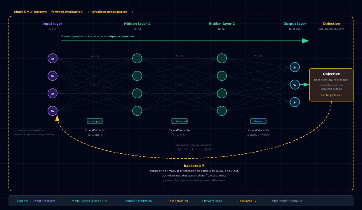
The architecture is Nets.FEED_FWD (nnx.FeedFwdNN): a 784-unit input layer (flattened MNIST), two hidden layers [256, 128] with ReLU, and a 10-unit output layer consumed by softmax + cross-entropy. The widths are deliberately generous for MNIST so the network has redundant capacity and the pruning curve is shallow through the mid-sparsity range.

Object	hidden_dims	Role
FP32 baseline	[256, 128]	Trained for 3 epochs; the pruning substrate
Pruned copies	[256, 128]	deepcopy of baseline, pruned at each \(s\)

The shared contract:

• Net: Nets.FEED_FWD, activation: Activations.RELU
• Loss: Losses.CROSS_ENTROPY
• Optimizer: Adam, max_lr=1e-3, weight_decay=0.0, momentum=(0.9, 0.999)
• Device: Devices.CPU
• Budget: N_EPOCHS=3 for the baseline
• Sparsity sweep: SPARSITY_LEVELS=[0.1, 0.3, 0.5, 0.7, 0.9] (or [0.1] under SMOKE_TEST=1)
• Pruning call: nnx.prune.magnitude_prune(net, sparsity=s) with bake=True (default) and layer_pattern="*" (all Linear layers)
• Seed: 0

The a priori expectation (against a well-trained baseline): accuracy is flat through \(s \le 0.5\), degrades slowly through \(0.5 \le s \le 0.7\), and drops sharply past \(s \approx 0.8\). The recorded run's baseline is undertrained (3 epochs, \(\sim 52\%\) val accuracy), so the absolute numbers are low and the curve is noisy in places — see results.

8.7.5 Code walkthrough

8.7.5.1 Baseline training

model = make_model()   # FeedFwdNN, [256, 128]
run = model.train(
    params=NNTrainParams(
        n_epochs=N_EPOCHS,
        train_loader=ds.train_loader, val_loader=ds.val_loader,
        optim=NNOptimParams(name=Optims.ADAM, max_lr=LR,
                            momentum=(0.9, 0.999), weight_decay=0.0),
    ),
)

The baseline trains for 3 epochs and reaches a final validation loss of 1.8857 (validation accuracy \(\sim 51.9\%\)). The short budget is a Tier-A choice (\(\sim 15\) s on CPU); the shape of the pruning curve is what is pedagogically interesting and it is stable across budgets, but the absolute accuracies are well below MNIST state-of-the-art.

8.7.5.2 Measuring the actual zero fraction

def actual_zero_fraction(net):
    total, zeros = 0, 0
    for p in net.parameters():
        if p.ndim < 2:
            continue           # skip biases; only count Linear weight matrices
        total += p.numel()
        zeros += (p == 0).sum().item()
    return zeros / total if total else 0.0

The ndim < 2 guard skips biases (1-D tensors) so the reported zero fraction is over Linear weight matrices only — the tensors magnitude pruning actually touches. This matters for reading the Pareto curve: a reported 50% zero fraction means 50% of weight entries, not 50% of all parameters including biases.

8.7.5.3 The sparsity sweep

for s in SPARSITY_LEVELS:
    pruned = copy.deepcopy(model)                       # start fresh from FP32 each time
    n_pruned = nnx_prune.magnitude_prune(pruned.net, sparsity=s)   # bake=True default
    edp = pruned.evaluate(ds.val_loader)
    zf = actual_zero_fraction(pruned.net)
    results.append((f"{s:.1f}", s, edp.accuracy, zf))

Three details. First, the baseline model is deepcopy'd at each \(s\), so every iteration starts from the same FP32 weights — the only thing varying across the sweep is \(s\). Second, magnitude_prune is called on pruned.net (the raw nnx.FeedFwdNN), not on the NNModel wrapper; it returns the number of layers that were pruned. Third, bake=True is the default, so after the call pruned.net's state_dict() has the same keys as the unpruned net, with physical zeros in the pruned positions — the deployable form.

8.7.5.4 The Pareto curve

ax.plot(xs, [a*100 for a in accs], "o-", label="val accuracy (%)", color="tab:blue")
ax2 = ax.twinx()
ax2.plot(xs, [z*100 for z in zfs], "s--", label="actual zero fraction (%)", color="tab:orange")

Accuracy on the left axis, actual zero fraction on the right, target sparsity on the horizontal. Overlaying both makes the "did we actually hit the target sparsity?" check visual — the orange dashed line should track the diagonal.

8.7.6 Results & analysis

On the recorded (seeded) run, the baseline and the five pruned points land as:

Target sparsity	Val accuracy	Actual zero fraction (Linear weights)
0.0 (baseline)	51.87%	0.00%
0.1	52.27%	10.00%
0.3	54.72%	30.00%
0.5	50.72%	50.00%
0.7	46.15%	70.00%
0.9	22.88%	90.00%

Three observations:

1. The actual zero fraction matches the target exactly (10.00%, 30.00%, 50.00%, 70.00%, 90.00%). This confirms the pruning contract: magnitude_prune(sparsity=s) produces a tensor that is \(s\)-sparse by construction, and bake=True writes those zeros permanently. The orange curve lies exactly on the diagonal.
2. Through \(s = 0.5\), accuracy is flat or even above the baseline (52.27%, 54.72%, 50.72% vs the 51.87% baseline). The \(s = 0.3\) point landing above the baseline is the non-monotonicity the notebook's §6.3 calls out: the 3-epoch baseline is itself noisy (\(\sim 52\%\)), so the absolute accuracies fluctuate within that noise band. Against a well-trained baseline the curve would be monotone with a crisp knee; the shape through mid-sparsity is the part that generalizes.
3. The cliff is at \(s \ge 0.8\). Accuracy holds at \(s = 0.7\) (46.15%, down ~6 points from baseline) then collapses to 22.88% at \(s = 0.9\) — the remaining 10% of weights cannot express the decision boundary. This is the "knee" the Pareto-curve framing predicts, and it is the deployment sweet-spot signal: for this architecture/dataset, prune to \(s \approx 0.7\) and stop.

The right reading: the zero-fraction-vs-target identity is the pruning contract (verified exactly), and the accuracy-vs-sparsity shape is budget-dependent in absolute terms but stable in shape — flat through mid-sparsity, cliff past ~0.8.

8.7.7 Pitfalls & edge cases

• 2:4 semi-structured sparsity is CUDA-only. nnx.prune.semi_structured_24 calls torchao's SparseSemiStructuredTensor, which requires CUDA-resident weights on NVIDIA Ampere-or-newer architectures. On CPU the swap raises RuntimeError at construction. This notebook is Tier-A / CPU-only, so the 2:4 path is mentioned in §6.3 but not exercised; the swap-mechanics contract is covered by the nnx test suite under a CUDA-available guard. Do not attempt to run it on the recommended CPU runtime.
• bake=True is a one-way door for continued training. Baking writes the zeros into .weight and drops the mask, so if you then resume training, the pruned weights will fill back in (no mask to hold them at zero). If you want to keep training the pruned model with the sparsity preserved (gradient-masking semantics), pass bake=False and PyTorch's pruning reparam stays in place. This notebook deploys the baked form; choose deliberately.
• The 3-epoch baseline is undertrained and noisy. Recorded val accuracy \(\sim 52\%\) is well below MNIST state-of-the-art, and the curve is non-monotonic through mid-sparsity (the \(s=0.3\) point lands above the baseline). Read the shape (flat → cliff), not the absolute numbers; a longer budget makes the curve monotone without changing the knee location.
• Skip biases when measuring zero fraction. magnitude_prune targets Linear weight matrices (2-D). The actual_zero_fraction helper guards on p.ndim < 2 to exclude biases; without that guard, the reported zero fraction is diluted by never-pruned bias entries and the "did we hit target sparsity?" check looks wrong.
• deepcopy the baseline per \(s\). Re-pruning the same model at escalating \(s\) without deepcopy would prune an already-pruned tensor, compounding sparsity and producing non-comparable points. The notebook copies fresh from the FP32 baseline each iteration.
• The knee is architecture- and dataset-dependent. The \(\sim 0.7\) knee reported here is for a [256, 128] FFN on MNIST. A larger model has more redundancy and tolerates higher \(s\); a smaller model hits the cliff sooner. Re-sweep before deploying the "prune to 0.7" heuristic on a different architecture.
• Quantization cousin (§8.8) is Tier B under Issue #66. This pruning notebook remains Tier A and covered by the 18-output oracle; the complete PTQ/QAT notebook runs in the bounded Tier B matrix with checkpoint reconstruction and semantic output verification.

8.7.8 Extensions & references

• Iterative (train-prune-retrain) pruning. This notebook does one-shot pruning on a trained baseline. The classical alternative is iterative magnitude pruning: prune a small fraction, retrain, prune again, repeat. This typically reaches higher final sparsity at the same accuracy because the model adapts to each pruning step. nnx.prune.magnitude_prune with bake=False supports the mask-preserving form needed for the retrain phase.
• Exercise 2:4 semi-structured sparsity on a GPU. Swap magnitude_prune for nnx.prune.semi_structured_24 on an Ampere+ CUDA runtime and measure the real wall-clock speedup from the sparse Tensor Cores. The contract is the same (a sparse deployable weight); the win is hardware acceleration rather than raw compression.
• Pair pruning with quantization (§8.8). Prune to \(s = 0.7\), then PTQ or QAT the pruned model. Sparse + int8 is the dominant edge-deployment recipe and the two nnx primitives compose cleanly; the joint Pareto curve (accuracy vs size vs latency over the \(s \times\) bitwidth grid) is the full deployment study.
• Structured (channel) pruning. Magnitude pruning is unstructured — any entry can be zeroed, so the speedup requires sparse kernels. Structured pruning removes whole channels/filters, producing a smaller dense model that is fast on any hardware. nnx does not currently ship a structured primitive; adding one would complete the pruning surface.
• References. Han et al., 2015, Learning both Weights and Connections for Efficient Neural Networks (arXiv:1506.02626) — the iterative train-prune-retrain recipe. Mishra et al., 2021, Accelerating Sparse Deep Neural Networks — the 2:4 semi-structured formulation backed by NVIDIA's SparseSemiStructuredTensor. See also the task README.md for the in-repo contract summary and docs/env-setup.md §4.1.6 for the Tier-A execution path.